Signal to Noise

The rms noise can be computed from

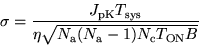$$\sigma = \frac{J_{\rm pK} T_{\rm sys}} {\eta \sqrt{N_{\rm a} (N_{\rm a}-1) N_{\rm c} T_{\rm ON} B}}$$ (1)

where

$\circ$

$T_{\rm sys}$ is the mean system temperature in $T_r^{*}$ scale (150K below 110GHz, 300K at 115GHz, 500K at 230GHz for sources at $\delta \ge 20^\circ$),

$\circ$

$J_{\rm pK}$ is the conversion factor from Kelvin to Jansky (22 at 3mm, 35 at 1.3mm),

$\circ$

$\eta$ is an efficiency factor due to atmospheric phase noise (0.9 at 3mm, 0.8 at 1.3mm),

$\circ$

$N_{\rm a}$ is the number of antennas (5), and $N_{\rm c}$ is the basic number of configurations (1 for D, 2 for CD, and so on)

$\circ$

$T_{\rm ON}$ is the integration time per configuration in seconds (2 to 8 hours, depending on source declination). Because of calibrations and antenna slew time, the effective (on-source) integration time is about 60-70% of the total observing time,

$\circ$

$B$ is the channel bandwidth in Hz (580 MHz for continuum, 40 kHz to 2.5 MHz for spectral line, according to spectral correlator setup).

Investigators have to specify the one sigma noise level which is necessary to achieve each individual goal of a proposal, and particularly for projects aiming at deep integrations.