


Next: 15.2 Sampling & Aliasing
Up: 15. The Imaging Principles
Previous: 15. The Imaging Principles
Contents
Subsections
The first step in imaging is to evaluate the dirty image,
using Fourier Transform. Several techniques are available.
The simplest approach would be to directly compute  and
and  functions
in Eq.15.4 for all combinations of visibilities and pixels in the image.
This is straightforward, but slow. For typical data set from the VLA, which
contain up to
functions
in Eq.15.4 for all combinations of visibilities and pixels in the image.
This is straightforward, but slow. For typical data set from the VLA, which
contain up to  visibilities per hour and usually require large images
(
visibilities per hour and usually require large images
(
 pixels), the computation time can be prohibitive. On the
other hand, the IRAM Plateau de Bure interferometer produces about
pixels), the computation time can be prohibitive. On the
other hand, the IRAM Plateau de Bure interferometer produces about  visibilities per synthesis,
and only require small images (
visibilities per synthesis,
and only require small images (
 ). The Direct Fourier Transform
approach could actually be efficient on vector computers for spectral line data
from Plateau de Bure interferometer, because the and functions needs to be evaluated only
once for all channels. Moreover, the method is well suited to real-time display,
since the dirty image can be easily updated for each new visibility.
). The Direct Fourier Transform
approach could actually be efficient on vector computers for spectral line data
from Plateau de Bure interferometer, because the and functions needs to be evaluated only
once for all channels. Moreover, the method is well suited to real-time display,
since the dirty image can be easily updated for each new visibility.
In practice, everybody uses the Fast Fourier Transform because of its definite
speed advantage. The drawback of the methods is the need to regrid the visibilities
(which are measured at arbitrary points in the  plane) on a regular
grid to be able to perform a 2-D FFT.
This gridding process will introduce some distortion in the dirty image and dirty
beams, which should be corrected afterwards. Moreover, the gridded visibilities
are sampled on a finite ensemble. As discussed in more details below, this sampling
introduces aliasing of the dirty image (and beam) in the map plane.
plane) on a regular
grid to be able to perform a 2-D FFT.
This gridding process will introduce some distortion in the dirty image and dirty
beams, which should be corrected afterwards. Moreover, the gridded visibilities
are sampled on a finite ensemble. As discussed in more details below, this sampling
introduces aliasing of the dirty image (and beam) in the map plane.
The goal of gridding is to resample the visibilities on a regular grid for
subsequent use of the FFT. At each grid point, gridding involves some sort
of interpolation from the values of the nearest visibilities. The visibilities
being affected by noise, the interpolating function needs not fit exactly
the original data points. Although any interpolation scheme could a priori
be used, such as smoothing spline functions, it is customary to use a
convolution technique to perform the gridding.
Using a convolution is justified by several arguments. First, from Eq.15.1,
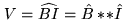 . Hence
  is already a convolution
of a (nearly Gaussian) function
is already a convolution
of a (nearly Gaussian) function  with the Fourier Transform of
  .
Nearby visibilities are not independent. Second, as mentioned above, exact
interpolation is not desirable, since original data points are noisy samples of
a smooth function. Third, if the width of the convolution kernel used in gridding
is small compared to , the convolution added in the gridding process will
not significantly degrade the information. Last, but not least, it is actually
possible to correct for the effects of the convolution gridding.
.
Nearby visibilities are not independent. Second, as mentioned above, exact
interpolation is not desirable, since original data points are noisy samples of
a smooth function. Third, if the width of the convolution kernel used in gridding
is small compared to , the convolution added in the gridding process will
not significantly degrade the information. Last, but not least, it is actually
possible to correct for the effects of the convolution gridding.
To demonstrate that, let  be the gridding convolution kernel.
Eq.15.3 becomes
be the gridding convolution kernel.
Eq.15.3 becomes
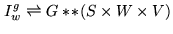 |
(15.6) |
We thus have for the image the following relations
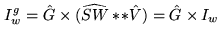 |
(15.7) |
and for the dirty beams
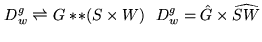 |
(15.8) |
from which we derive the relation
 |
(15.9) |
Thus the dirty image and dirty beams are obtained by dividing the Fourier Transform
of the gridded data by the Fourier Transform of the gridding function.
Next: 15.2 Sampling & Aliasing
Up: 15. The Imaging Principles
Previous: 15. The Imaging Principles
Contents
Anne Dutrey