6.3 The Correlator in Practice

In order to numerically evaluate the cross-correlation function $R_{\rm ij}$, the continuous signals entering the cross correlator need to be sampled and quantized. According to Shannon's sampling theorem [Shannon 1949], a bandwidth-limited signal may be entirely recovered by sampling it at time intervals $\Delta t \le 1/(2\Delta\ensuremath{\nu_\mathrm{\scriptscriptstyle IF}})$ (also called sampling at Nyquist rate). The discrete Fourier transform of the sufficiently sampled cross-correlation function theoretically yields the cross-power spectrum without loss of information. However, in practice, two intrinsic limitations exist:

• In order to discretize a signal, it is not only sampled, it also has to be quantized. The cross-correlation function, as derived from quantized signals, does not equal the cross-correlation function of continuous signals. Moreover, the sampling theorem does not hold anymore for quantized signals. The reasons will become clear below.
• Eq.6.7 theoretically extends from $-\infty$ to $+\infty$. In practice (Eq.6.8), only a maximum time lag can be considered: limited storage capacities and digital processing speed are evident reasons, another limiting factor are the different timescales mentioned before. The abrupt cutoff of the time window affects the data.

These ``intrinsic'' limitations are discussed in Sections 6.3.1 and 6.3.2. The system-dependent performance will be addressed in Section 6.3.3.

6.3.1 Digitization of the input signal and clipping correction

As already mentioned, sampling at the Nyquist rate retains all information. However, quantizing the input signal leads to a loss of information. This can be qualitatively understood in the following way: in order to reach the next discrete level of the transfer function, some offset has to be added to the signal. If the input signal is random noise of zero mean, the offset to be added will also be a random signal of zero mean. In other words, a ``quantization'' noise is added to the signal, that leads to a loss of information. In addition, the added noise is not anymore bandwidth limited, and the sampling theorem does not apply: oversampling will lead to improved sensitivity.

Many quantization schemes exist (see e.g. [Cooper 1970]). It is entirely sufficient to use merely a few quantum steps, if the cross-correlation function will be later corrected for the effects of quantization. For the sake of illustration, the transfer function of a four-level 2-bit quantization is shown in Fig.6.5. Each of the four steps is assigned a sign bit, and a magnitude bit. After discretizing the signal, the samples from one antenna are shifted in time, in order to compensate the geometric delay $\ensuremath{\tau_\mathrm{\scriptscriptstyle \rm G}}(t)$. The correlator now proceeds in the following way: for each delay step $\Delta t$, the corresponding sign and magnitude bits are put into two registers (one for the first antenna, and one for the second). The second register is successively shifted by one sample. In this way, sample pairs from both antennas, separated by a successively longer time lag, are created. These pairs are multiplied, using a multiplication table. For the case of four-level quantization, it is shown in Fig.6.5. Products which are assigned a value of $\pm{n}^2$ are called ``high-level products'', those with a value of $\pm{n}$ are ``intermediate-level products'', and those with a value of $\pm{1}$ ``low-level products''. The products (evaluated using the multiplication table in Fig.6.5) are sent to a counter (one counter for each channel, i.e. for each of the discrete time lags). After the end of the integration cycle, the counters are read out.

In practice, the multiplication table will be shifted by a positive offset of $n^2$, to avoid negative products (the offset needs to be corrected when the counters are read out). This is because the counter is simply an adding device. As another simplification, low-level products may be deleted. This makes digital implementation easier, and accounts for a loss of sensitivity of merely 1% (see Table 6.1). Finally, not all bits of the counters' content need to be transmitted (see Section 6.3.2).

Before the normalized contents of the counters are Fourier-transformed, they need to be corrected, because the cross-correlation function of quantized data does not equal the cross-correlation function of continuous data. This ``clipping correction'' can be derived using two different methods. As an example for the case of full 4-level quantization:

• Four-level cross-correlation coefficient according to the multiplication table Fig.6.5. The cross-correlation coefficient $\rho$ is a normalized form of the cross-correlation function (see AppendixA):

  $$\rho_4 = \frac{2n^2(N_{01,01}-2N_{01,11})+4n(N_{00,01}-N_{00,11}) +2(N_{00,00}-N_{00,10})}{2(n^2N_{01,01}+N_{00,00})_{\rho = 1}}$$ (6.8)

  
  
  where $N_{\rm ij,kl}$ is the number of counts with sign bit $i$ and magnitude bit $j$ at time $t$ (first antenna), and sign bit $k$ and magnitude bit $l$ at time $t+\tau$ (second antenna). $\pm{n}$ is the product value assigned to intermediate-level products.
• Clipping correction, first method: evaluate the $N_{\rm ij,kl}$ in Eq.6.9, using joint probabilities $P_{\rm ij,kl}$ (see AppendixA for the definition of the jointly Gaussian probability distribution), such as

  $$N_{01,01} = NP_{01,01} = \frac{N}{2\pi\sigma^2\sqrt{1-\rho^2}} \i... ...nfty}{ \exp{\left[\frac{-(x^2+y^2-2\rho xy)}{2\sigma^2(1-\rho^2)}\right]}dx}dy}$$ (6.9)

  
  
  ($N$ is the number of signal pairs, separated by the time lag of the channel under consideration, $v_0$ is the clipping voltage, see Fig.6.4).
• Clipping correction, second method: using Price's theorem for functions of jointly random variables. The result, derived in AppendixB, is shown in Fig.6.4:
  

  $$R_4 = \frac{\sigma^2}{\pi}\int_{0}^{\rho}{ \frac{1}{\sqrt{1-r^2}}\biggl... ...\sigma^2(1+r)}\right)}+ \exp{\left(\frac{-v_0^2}{\sigma^2(1-r)}\right)}\right]}$$

  $${+4(n-1)\exp{\left(\frac{-v_0^2}{2\sigma^2(1-r^2)}\right)}+2\biggr\}dr} .$$ (6.10)

  
  

Although the discrete, normalized cross-correlation function and the continuous cross-correlation coefficient are almost linearly dependent within a wide range, the correction is not trivial. An analytical solution is only possible for the case of two-level quantization (``van Vleck correction''  [Van Vleck 1966]).

In practice, several methods are used to numerically implement Eq.6.11 (in the following, the index $k$ means k-level quantization). The integrand may be replaced by an interpolating polynomial, allowing to solve the integral. One may also construct an interpolating surface $\rho(R_{\rm k},\sigma)$. As already discussed, the clipping correction cannot recover the loss of sensitivity due to quantization. The loss of sensitivity for $k$-level discretization may be found by evaluating the signal-to-noise ratio

$$\Re_{{\rm sn},k}= \frac{R_{\rm k}}{\sigma_k} = \frac{R_{\rm k}}{\sqrt{\langle R_k^2\rangle - \langle R_k \rangle^2}}$$ (6.11)

In order to minimize the loss of sensitivity, the clipping voltage (with respect to the noise $\sigma$) needs to be adjusted such that the correlator efficiency curve in Fig.6.4 is at its maximum. The correlator efficiency is defined with respect to the signal-to-noise ratio of a (fictive) continuous correlator, i.e.

$$\eta_k = \frac{\Re_{{\rm sn},k}}{\Re_{\rm sn,\infty}} = \frac{\Re_{{\rm sn},k}}{\rho\sqrt{N_{\rm q}}}$$ (6.12)

where $N_{\rm q}$ is the number of samples. Table6.1 summarizes the results for different correlator types and samplings.


Due to the discretization of the input voltages (as shown in Fig.6.5), any knowledge of the absolute signal value is lost. The signal amplitude is recovered by a regularly performed calibration (using a calibration load of known temperature, for details, see Chapter 12 by A.Dutrey). Fig.6.6 shows the signal processing steps from the incoming time series to the derived spectrum.

Figure 6.4: Left: Clipping correction (cross correlation coefficient of a continuous signal vs. cross correlation correlation coefficient of a quantized signal) for two-, three- and four level quantization (with optimized threshold voltage). The case of two level quantization is also known as van Vleck correction. For more quantization levels, the clipping correction becomes smaller. Right: Correlator efficiency as function of the clipping voltage, for three-level and four-level quantization (at Nyquist sampling).

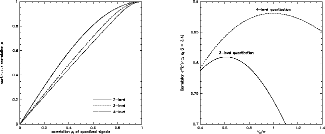Figure 6.5: Left: Transfer function for a 4-level 2-bit correlator. The dashed line corresponds to the transfer function of a (fictive) continuous correlator with an infinite number of infinitesimally small delay steps. Right: Multiplication table. $S(x)$ is the signal bit at time $t$, $M(x)$ is the magnitude bit at time $t$ (respectively $S(y)$ and $M(y)$ at time $t+\tau$).

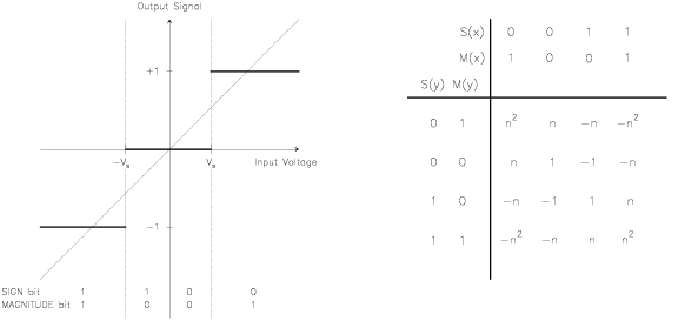Figure 6.6: The signal processing in a 3-level 2-bit correlator. From top to bottom: the original time series (sampled in discrete time steps, but continuous in amplitude), the digitized time series (with high-level weight 3), the digital correlation $R_4$, the reconstructed spectral line.

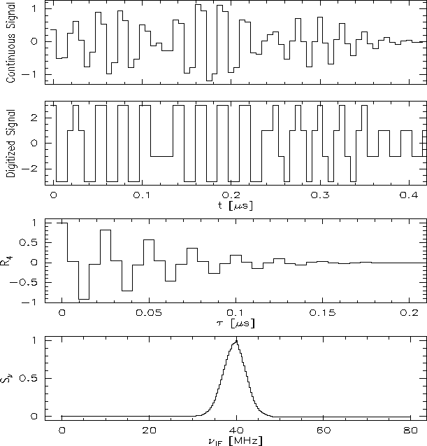Table 6.1: Correlator parameters for several quantization schemes

method	$n$	$v_0$ [ $\sigma_{\rm rms}$]	$\eta_{\rm q}^{(1)}$ for
			sampling rate
			$2\Delta\ensuremath{\nu_\mathrm{\scriptscriptstyle IF}}^{(2)}$	$4\Delta\ensuremath{\nu_\mathrm{\scriptscriptstyle IF}}^{(3)}$
two-level	-	-	0.64	0.74
three-level	-	0.61	0.81	0.89
four-level	3	1.00	$0.88^{(4)}$	0.94
	4	0.95	0.88	0.94
$\infty$-level	-	-	1.00	1.00

Notes:
(1) The correlator efficiency is defined by Eq.6.13.
The values are for an idealized (rectangular)
bandpass and after level optimization.
(2) Nyquist sampling,
(3) oversampling by factor 2
(4) 0.87 if low level products deleted
(case of Plateau de Bure correlator)

Table 6.2: Time lag windows

Description	Lag window	Spectral window
rectangular	$w(t) = 1$ for $\vert t\vert \le \tau_{\rm m}$, else 0	$\hat{w}(\nu) = 2\tau_{\rm m}\frac{\sin{(2\pi\nu \tau_{\rm m})}}{2\pi\nu\tau_{\rm m}}$
Bartlett	$w(t) = 1-\frac{\vert t\vert}{\tau_{\rm m}}$ for $\vert t\vert \le \tau_{\rm m}$, else 0	$\hat{w}(\nu) = \tau_{\rm m} \left(\frac{\sin{(\pi\nu\tau_{\rm m})}}{\pi\nu\tau_{\rm m}}\right)^2$
von Hann	$w(t) = \frac{1}{2}\left(1+\cos{(\frac{\pi t}{\tau_{\rm m}})} \right)$ for $\vert t\vert \le \tau_{\rm m}$, else 0	$\hat{w}(\nu) = \tau_{\rm m}\cdot\frac{\sin{(2\pi\nu\tau_{\rm m})}} {2\pi\nu\tau_{\rm m}}\cdot\frac{1}{1-(2\nu\tau_{\rm m})^2}$
Welch	$w(t) = \left(1-(\frac{t}{\tau_{\rm m}})^2\right)$	$\hat{w}(\nu) = \frac{1}{(\pi\nu)^2\tau_{\rm m}}\left( \frac{\sin{(2\pi\nu\tau_... ...nu\tau_{\rm m}}-{\mbox{\small cos}\mbox{\small $(2\pi\nu\tau_{\rm m})$}}\right)$
Parzen	$w(t) = \left\{ \begin{array}{l} 1-6\left(\frac{t}{\tau_{\rm m}}\right)^2+6\lef... ...thrm{for}    \tau_{\rm m}/2 < \vert t\vert \le \tau_{\rm m} \end{array}\right.$	$\hat{w}(\nu) = \frac{3}{4}\tau_{\rm m} \left(\frac{\sin{(\pi\nu\tau_{\rm m}/2)}}{\pi\nu\tau_{\rm m}/2}\right)^4$

6.3.2 Time lag windows and spectral resolution

According to the sampling theorem, we need a sampling timestep $\Delta t = 1/(2\Delta\ensuremath{\nu_\mathrm{\scriptscriptstyle IF}})$ if we want to fully recover the cross-power spectral density within a bandwidth $\Delta\ensuremath{\nu_\mathrm{\scriptscriptstyle IF}}$. The channel spacing $\delta\nu$ is then determined by the maximum time lag $\tau_{\rm max} = N_{\rm ch}\Delta t$ (where $N_{\rm ch}$ is the number of channels), i.e.

$$\delta\nu = \frac{1}{2\tau_{\rm max}} = \frac{1}{2N_{\rm ch}\Delta t}$$ (6.13)

However, the data acquisition is abruptly stopped after the maximum time lag. After the Fourier transform, the observed cross power spectrum is thus convolved with the Fourier transform $\hat{w}(\nu)$ of the box-shaped time window $w(t)$, producing strong sidelobes:

$$w(\tau) = \left\{ \begin{array}{ll} 1, & \vert\tau\vert \le \tau_... ...au_{\rm max})}}{2\ensuremath{\nu_\mathrm{\scriptscriptstyle }}\tau_{\rm max}}\;$$ (6.14)

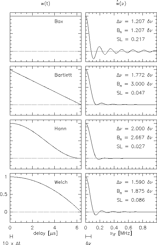
These oscillations are especially annoying, if strong lines are observed. They may be minimized, if the box-shaped time lag window is replaced by a function that rises from zero to peak at negative time lags, and decreases to zero at positive time lags (apodization). Such a window function suppresses the sidelobes, at the cost of spectral resolution. A comparison between several window functions is given in Fig.6.7, together with sidelobe levels and spectral resolutions (defined by the full width at half-power, FWHP, of the main lobe of the spectral window). 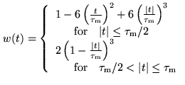Table 6.2 summarizes the various functions in time and spectral domains. The default of the Plateau de Bure correlator is the Welch window, because it still offers a good spectral resolution. Moreover, the oscillating sidelobes partly cancel out the contamination of a channel by the signals in adjacent channels. Of course, the observer is free to deconvolve the spectra from this default window, and to use another time lag window.
Note: If you apodize your data, not only the effective spectral resolution is changed. Due to the suppression of noise at large time lags, the sensitivity is increased. The variance ratio of apodized data to unapodized data,

$$\int_{-\infty}^\infty{\vert w(t)\vert^2dt} = \int_{-\infty}^\infty{\vert\hat{w}(\nu)\vert^2d\nu} = 1/B_{\rm n}$$ (6.15)

defines the noise equivalent bandwidth $B_{\rm n}$. It is the width of an ideal rectangular spectral window (i.e. $\hat{w}(\nu) = 1/B_{\rm n}$ with zero loss inside $\vert\nu\vert \le B_{\rm n}/2$, and infinite loss outside) containing the same noise power as the actual data. For sensitivity estimates of spectral line observations, the channel width to be used is thus the noise equivalent width, and neither the channel spacing, nor the effective spectral resolution. Fig.6.7 gives the noise equivalent bandwidths $B_{\rm n}$ for commonly used time lag windows.

Figure: Several time lag windows, and their Fourier transforms (normalized to peak). The sidelobe levels SL are indicated, as well as the spectral resolution (defined as the FWHP of the main lobe), and the noise equivalent width. The delay stepsize, and channel spacing are indicated for the following example: 256 channels, clock rate 40MHz, resulting in a channel spacing of 78.125kHz.

6.3.3 Main limitations

In real life, cross-correlators are subject to the performance of the whole receiving system. This comprises the ``analog part'' (the signal path from the receivers to the IF filters at the correlator entry), and the ``digital part'' (everything behind the sampler). Although the analog part is out of the correlator, its performance requires to change our assumptions concerning the input data. This complicates the analysis of the correlator response. The following discussion refers to instantaneous errors only. However, in interferometric mapping, scan-averaged visibilities are used, and the data may be less affected.

6.3.3.1 Analog part

The shape of the bandpass function (amplitude and phase) at the correlator output is mainly due to the correlator's response to the filters inserted in the IF band at the correlator entry. So far, for the sake of simplicity, rectangular passbands, centered at the intermediate frequency $\ensuremath{\nu_\mathrm{\scriptscriptstyle IF}}$, have been assumed. A more complex (and more realistic) case may be an amplitude slope where the logarithm of the amplitude varies linearly with frequency. Although the bandpass function will be calibrated (see Eq.6.17, and R.Lucas Chapter 7), the effect of such a slope on sensitivity remains. A derivation of the signal-to-noise ratio for that case is beyond the scope of this lecture. To give an impression of the order of magnitude: a slope of 3.5dB (edge-to-edge) leads to a 2.5% degradation of the sensitivity calculated for a rectangular passband. A center frequency displacement of 5% of the bandwidth leads to the same degradation.

As already demonstrated, delay-setting errors linearly increase with the intermediate frequency (Eq.6.6). Table6.3 gives an impression of the decrease of sensitivity due to a delay error. The effect is also shown in Fig.6.3 for a range of delay errors. For example, a delay error of $0.12/\Delta\ensuremath{\nu_\mathrm{\scriptscriptstyle IF}}$ accounts for a 2.5% degradation. Delay errors are mainly due to inaccurately known antenna positions (asking for a better baseline calibration), or due to errors in the transmission cables.

Table 6.3: Effects of delay pattern on the sensitivity

Intermediate frequency bandwidth	$\ensuremath{\nu_\mathrm{\scriptscriptstyle IF}} = 160$MHz
Baseline	$b = 100$m
Zenith distance of source in direction $\ensuremath{\text{\boldmath $s$\unboldmath }}$	$\Theta = 30^\circ$
Results in geometric delay:	$\ensuremath{\tau_\mathrm{\scriptscriptstyle \rm G}} = \ensuremath{\text{\boldm... ...\unboldmath }}\cdot \ensuremath{\text{\boldmath $s$\unboldmath }}/c = 0.17 \mu$s
Attenuation according to Eq.6.4	$1 \%$

Phase errors across the bandpass may also be of random nature. A phase fluctuation of $12.8^\circ$ (rms) per scan leads to a degradation of $(1-\exp{(-\sigma_\Phi^2/2)}) \times 100 \% = 2.5 \%$.

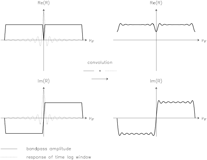
Figure 6.8: The Gibbs phenomenon. The convolution of the bandpass with the (unapodized) spectral window (sinc function) is shown for the real and imaginary parts. Note that for the real part, the phenomenon is stronger at the band edges, whereas for the imaginary part, it contaminates the whole bandpass.

Fluctuations across the bandpass also appear as ripples. They may have several reasons, and are mainly due to the Gibbs phenomenon, and due to reflections in the transmission cables. A sinusoidal bandpass ripple of 2.9dB (peak-to-peak) yields a 2.5% degradation in the signal-to-noise ratio. The Gibbs phenomenon also occurs in single-dish autocorrelation spectrometers. For the sake of illustration, let us again assume a perfectly flat response of receivers and filters. However, the filter response function is only flat across the IF passband. Towards its boundary, steep edges occur. We already learned that strong spectral lines may show ripples, if no special data windowing in time domain is applied. The Gibbs phenomenon is due to a similar problem (but now the spectral line is replaced by the edge of a flat rectangular band extending in frequency from zero to $\Delta\ensuremath{\nu_\mathrm{\scriptscriptstyle IF}}$). The output of the cosine correlator is symmetric, but the sine output (imaginary part) is antisymmetric, thus including an even steeper edge. Convolving this edge with the sinc function (i.e. the spectral window) results in strong oscillations. Let us call this function $f(\nu)$. For calibration purposes, the Gibbs phenomenon has to be avoided: the problem is that calibration uses the system response to a flat-spectrum continuum source. A source whose visibility is $V(\nu)$ is seen as $f(\nu) \ast [G_{\rm ij}(\nu)V(\nu)]$ (where $G_{\rm ij}$ is now a frequency-dependent complex gain function). After calibration it becomes

$$\hat{V}(\nu) = \frac{f(\nu)\ast [G_{\rm ij}(\nu)V(\nu)]}{f(\nu) \ast G_{\rm ij}(\nu)}$$ (6.16)

Due to the convolution product the complex gain $G_{\rm ij}(\nu)$ does not cancel out, as desired, and $\hat{V}(\nu) \ne V(\nu)$. Automatic calibration procedures have to flag the channels concerned. As shown in Fig.6.8, for the real part, the effect is stronger at the band edges, but the output of the imaginary part also shows ripples in the middle of the band (thus, the problem is of greater importance for interferometers than for single-dish telescopes using auto-correlators). If the bandwidth to be observed is synthesized by two adjacent frequency windows, the phenomenon is stronger at the band center. You should avoid to place your line there, if it is on top of an important continuum (see Section 6.4.1 for the case of the Plateau de Bure system).

The above summary of the system-dependent performance of a correlator is not exhaustive. For example, the phase stability of tunable filters, which depends on their physical temperature, is not discussed. Alternatives to such filters are image rejection mixers (as used in the Plateau de Bure correlator).

6.3.3.2 Digital part

Errors induced by the digital part are generally negligible with respect to the analog part. In digital delays, a basic limitation is given by the discrete nature of the delay compensation, which accuracy in turn is limited by the clock period of the sampler. However, digital techniques allow for high clock rates, keeping this error at a minimum.

Evidently, a basic limitation is given by the memory of the counters, setting the maximum time lag (which in turn defines the spectral resolution, as already discussed): with $2K$ bits, we can exactly represent $N=2^{2K}$ numbers. However, the information contained in the bits is not equivalent. For the 3-level 2-bit correlator, the output of each channel $i=1,...,N$ is

$$R(i) = \frac{1}{2}\left(N \pm \sqrt{N}\sqrt{1-{\rm erf} {\left(v_0/\sqrt{2}\right)}}\right)$$ (6.17)

(assuming white, Gaussian noise of zero mean and of unit variance, and neglecting the weak contribution of the astrophysical signal). The $1 \sigma$-precision of the output is $\approx \sqrt{N}/2$, contained in the last $K-1$ bits, which thus do not need to be transmitted. The maximum integration time before overflow occurs is set by the number of bits of the counter, and the clock frequency. Table6.4 shows an example.

Table 6.4: Maximum integration time of a 16-bit counter

clock frequency:	80MHz
weight for intermediate-level products:	$n = 3$
positive offset:	$n^2 = 9$
weight for autocorrelation product:	18 (using offset multiplication table)
carry out rate of a 4-bit adder	$18/2^4 = 1.125$
maximum integration time:	$2^{16}/(80$MHz$\times 1.125) = 0.73$ms
same with a 4-bit prescaler:	$2^{16}\times 2^4/(80$MHz$\times 1.125) = 11.7$ms

The only error cause due to the correlator that is worth to be mentioned is the sampler, i.e. the analog-to-digital conversion. As already shown, the threshold levels are adjusted with respect to the noise in the unquantized signal. However, the noise power may change during the integration. In that case, the correlator does not operate anymore at its optimum level (see Fig.6.4). This error cause can be eliminated with an automatic level control circuit. However, slight deviations from the optimal level adjustment may remain. Without going too far into detail, the deviations can be decomposed in an even and an odd part: in one case, the positive and negative threshold voltages move into opposed directions (even part of the threshold error). The resulting error can be equivalently interpreted as a change of the signal level with respect to the threshold $v_0$, and leads to a gain error. In the other case, the positive and negative threshold voltages move into the same direction (odd part of the threshold error). This error, however, can be reduced by periodic sign reversal of the digitized samples (if the local oscillator phase is simultaneously shifted by $\pi$, the correlator output remains unaffected). Combining the original and phase-shifted outputs, the error cancels out with high precision. Such a phase shift is implemented in the first local oscillators of the Plateau de Bure system (for details see Chapter 7 by R.Lucas). Note also that threshold errors of up to 10% can be tolerated without degrading the correlator sensitivity too much: the examination of Fig.6.4 shows that such an error results in a signal-to-noise degradation of less than 0.2% for a 3-level system, and of less than 0.5% for a 4-level system (the maxima of the efficiency curves are rather broad).


Another problem is that the nominal and actual threshold values may differ. The error can be described by ``indecision regions''. By calculating the probability that one or both signals of the cross-correlation product fall into such an indecision region, the error can be estimated. With an indecision region of 10% of the nominal threshold value, the error is negligibly small.


Finally, it should be noted that strict synchronisation of the time series from different antennas is mandatory: any deviation will introduce a phase error.