


Next: 16.3 Experimental data space
Up: 16. Advanced Imaging Methods:
Previous: 16.1 Introduction
Contents
In the problems of Fourier synthesis encountered in astronomy,
the object function of interest,
 , is a
real-valued function of an angular position variable
, is a
real-valued function of an angular position variable
 . The geometrical elements
under consideration are presented in Fig. 16.1.
. The geometrical elements
under consideration are presented in Fig. 16.1.
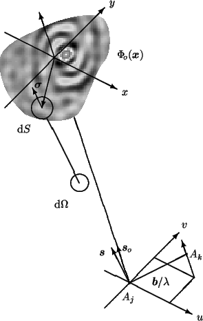
Figure 16.1:
Traditional coordinate systems used to express the
relation between the complex visibilities and the brightness distribution
of a source under observation. Here, the two antennas  and
and  point toward a distant radio source in a direction indicated by the
unit vector
point toward a distant radio source in a direction indicated by the
unit vector
 , and
, and
 is the interferometer baseline
vector. The position pointed by the unit vector
is the interferometer baseline
vector. The position pointed by the unit vector
 is commonly
referred to as the phase tracking center or phase reference
position:
is commonly
referred to as the phase tracking center or phase reference
position:
 .
.
 |
The object model variable  lies in some
object space
lies in some
object space  whose vectors, the functions ,
are defined at a high level of resolution. This space
is characterized by two key parameters: the extension
whose vectors, the functions ,
are defined at a high level of resolution. This space
is characterized by two key parameters: the extension
 of its field, and its resolution scale
  .
To define this object space more explicitly, we first
introduce the finite grid (see Fig. 16.2):
.
To define this object space more explicitly, we first
introduce the finite grid (see Fig. 16.2):
 |
(16.1) |
where  is some power of
  .
.
On each pixel
 , we
then center a scaling function of the form
, we
then center a scaling function of the form
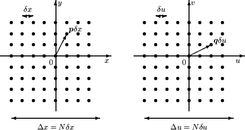
Figure:
Object grid
 (left hand)
and Fourier grid
(left hand)
and Fourier grid
 (right hand) for
  .
The object domain is characterized by its resolution scale
and the extension of its field
.
The object domain is characterized by its resolution scale
and the extension of its field
 , where is
some power of (the larger is , the more oversampled is the object
field). The basic Fourier sampling interval is
, where is
some power of (the larger is , the more oversampled is the object
field). The basic Fourier sampling interval is
 ,
the extension of the Fourier domain is
,
the extension of the Fourier domain is
 .
.
 |
It is easy to verify that these functions form an orthogonal set.
In this presentation of WIPE, the object space
is the Euclidian space generated by the basis vectors
 ,
,
 spanning
 (see Fig. 16.2). The dimension of
this space is equal to
(see Fig. 16.2). The dimension of
this space is equal to  : the number of pixels in the
grid
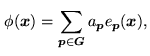
. The functions lying in can therefore
be expanded in the form
: the number of pixels in the
grid
. The functions lying in can therefore
be expanded in the form
 |
(16.3) |
where the
 's are the components of in the
interpolation basis of .
's are the components of in the
interpolation basis of .
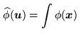
The Fourier transform of is defined by the relationship
 e e |
|
where
 is a two-dimensional angular spatial frequency:
 . According to the expansion of we therefore
have:
. According to the expansion of we therefore
have:
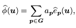 |
(16.4) |
where
 e e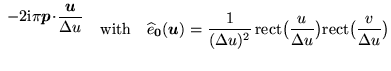 |
(16.5) |
and
.
The dual space of the object space,
 , is the
image of by the Fourier transform operator:
is
the space of the Fourier transforms of the functions lying
in .
This space is characterized by two key parameters: its
extension
, and the basic Fourier sampling
interval
(see Fig. 16.2).
, is the
image of by the Fourier transform operator:
is
the space of the Fourier transforms of the functions lying
in .
This space is characterized by two key parameters: its
extension
, and the basic Fourier sampling
interval
(see Fig. 16.2).
Next: 16.3 Experimental data space
Up: 16. Advanced Imaging Methods:
Previous: 16.1 Introduction
Contents
Anne Dutrey