18.2 Photometry

18.2.1 From Flux density to Brightness temperature

The unit of the dirty map is ill defined. A single point source of 1 Jy appears with peak intensity of 1. But if more than 1 point source is in the field of view, the combination of positive or negative sidelobes from the other source modifies this result. It is thus necessary to deconvolve. After deconvolution, the beam area is well defined: the CLEAN map unit is Jy per beam area.

The conversion to brightness temperature can then be done using the standard equation

$$S_\nu = \frac{2 k \ensuremath{\Omega_\mathrm{\scriptscriptstyle s}}}{\lambda^2} T_B$$ (18.1)

$$= \frac{2 k \pi \ensuremath{\theta_\mathrm{\scriptscriptstyle s}}^2}{4 \log{2} \lambda^2} T_B$$ (18.2)

for Gaussian beams. GO MAP and its variants automatically display the Jy/K conversion factor mentioned above. The integrated flux density in a user defined area can then be computed on the clean map using command GO FLUX.

18.2.2 Accuracy of Flux density estimates

The accuracy of flux measurements is limited by several factors.

Figure 18.1: Illustration of the difficulty to deconvolve a weak, extended structure. In this 1-D example, half of the flux is in the extended structure, and cannot be recovered properly by deconvolution because of low signal to noise.

Deconvolution Errors and Missing Flux

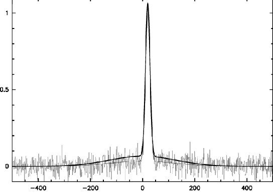
Deconvolution limits are among the most important. Deconvolution is required (see Chapter 15), but it is impossible to deconvolve weak structures near the noise level. Nevertheless, these structures, when sufficiently extended, can contribute to a significant flux. The relevance of the missing flux to the astronomical interpretation is to be decided by the astronomer. In most cases, however, the missing flux does not correspond to any significant brightness, and its absence may not modify the astronomical interpretation. A schematic illustration is given in Fig.18.1: half of the flux is buried in the noise, but the brightness is measured properly (within the statistical error). Note also that WIPE ([Lannes et al. 1997]) offers an upper limit to the noise amplification factor due to the non linear deconvolution process. This upper limit is often discouragingly large for the rather poor dirty beams provided by current mm arrays (4 or 5 is not unusual).

Comparing the recovered flux to a single dish measurement can help you in estimating the corresponding brightness level and evaluate whether this is important in your astronomical case. To convert from flux to brightness, the characteristic size of the missed flux should be used. This is in between several synthesized beam widths and about half of the primary beam. Although in general the problem is not as severe as one would think (because, unfortunately, one is often signal to noise limited), this is an important information, specially in the case of mosaics.

Seeing

A second important effect which affects flux density measurements is the seeing. Seeing result in an underestimation of Point source flux. On the other hand, the total flux is spread over the seeing disk, and is in principle conserved. Insufficient seeing conditions limit the deconvolution process, since the effective synthesized beam (which should include atmospheric phase errors) is significantly different from the theoretical synthesized beam (computed from $uv$ coverage and weights). A good check is to make an image of the two calibrators, and measure the corresponding point source flux and apparent size.

Noise estimate

Finally, the noise should be estimated. GO RMS gives the sigma of the image flux density distribution. This is an improper estimate, since it includes any possible signal, all spectral channels, and map edges where the noise level increases due to aliasing and gridding. A better estimate, derived from effective weights, is in principle given by task UV_STAT. However, this estimate does not take into account possible deconvolution problems or dynamic range limitations due to atmospheric phase noise. The optimal procedure is to use command GO FLUX on an empty area of the image to find out the point source rms noise. The precision of the estimate is limited by statistical uncertainties linked to the number of beams in the area. Then, another GO FLUX command on the emission area will give the total flux and number of independent beams, $n$; the rms on the total flux is $\sqrt{n}$ times the point source rms determined by the GO FLUX command applied to an empty region. Another good method to determine the noise level (yet to be implemented as a GO NOISE procedure...) would be to build the histogram of the pixel values and fit a Gaussian to it; if source structure only covers a small fraction of the image, this method provides a good estimate.

Primary beam

One should emphasize that primary beam correction is essential in any correct flux density estimate. All image plane analysis should be carried out on a primary beam corrected image. This introduces a slight complication, since the noise level is then not uniform. The GO FLUX commands discussed before should be applied in regions of similar extent and location vis-a-vis the primary beam(s).

$uv$ plane analysis is also extremely useful both in measuring integrated flux densities and rms noise level, at least for simple, relatively compact, source models. Task UV_FIT provides statistical errors for all parameters of the fit. Primary beam correction should be applied a posteriori, based on the location of the region of interest.

Dynamic Range

As mentioned above, the dynamic range may be a limitation. The dynamic range $D_r$ is defined as the ratio of the peak intensity to the lowest ``believable'' contour. $D_r$ is obviously lower than the signal to noise ratio. It can be estimated as the absolute value of the peak to maximum negative contour ratio. As usual, map edges should not be included in this evaluation. Dynamic range is related to seeing and calibration errors. It is typically 10 to 40 at Plateau de Bure (if signal to noise ratio allows). Errors should include dynamic range effects.

Flux density scale

Finally, remember that the flux scale is determined by bootstrapping flux of (variable) quasars from that of reference sources. Any errors accumulated in this process must be transferred to the source flux estimate.

In summary, flux density estimates should quote errors which include

• Effective thermal noise
• Dynamic range problems
• Relative (calibrator) flux uncertainty
• Absolute flux scale uncertainty  OR  reference flux scale.
• Primary beam correction