20.1 Introduction and Basic Formalism

Modern astrometry aims at improving our knowledge of celestial body positions, motions and distances to a high accuracy. The quest for accuracy began in the early days of astronomy and is still continuing in the optical domain with most sophisticated instruments (automated meridian circles, the Hipparcos satellite or future astrometric space missions) as well as in the radio domain (connected-element interferometers and VLBI). New instrumental concepts or calibration procedures and increased sensitivity are essential to measure highly accurate positions of stars and radio sources. Positions accurate to about one thousandth to one tenth of an arcsecond have now been obtained for hundreds of radio sources and for about 100 000 to one million stars in the Hipparcos and Tycho catalogues respectively.

In this lecture we are concerned with some basic principles of position measurements made with synthesis radio telescopes and with the IRAM interferometer in particular. More details on interferometer techniques can be found in the fundamental book of [Thompson et al. 1986]. The impact of VLBI in astrometry and geodesy is not discussed here. (For VLBI techniques see [Sovers et al. 1998].)

We first recall that measuring a position is a minimum prerequisite to the understanding of the physics of many objects. One example may be given for illustration. To valuably discuss the excitation of compact or masing molecular line sources observed in the direction of late-type stars and HII regions sub-arcsecond position measurements are required. This is because the inner layers of circumstellar envelopes around late-type stars have sizes of order one arcsecond or less and because several compact HII regions have sizes of one to a few arcseconds only. Position information is crucial to discuss not only the respective importance of radiative and collisional pumping in these line sources but also the physical asssociation with the underlying central object.

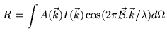
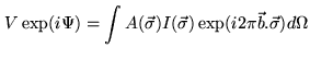
The output of an interferometer per unit bandwidth at the observing wavelength $\lambda$ is proportional to the quantity

$$R = \int A({\vec k}) I({\vec k}) \cos (2\pi {\vec {\cal B}}.{\vec k} / \lambda) d\Omega$$ (20.1)

where ${\vec k}$ is the unit vector toward the observed source, $A$ is the effective antenna aperture, $I$ the source brightness, and ${\vec {\cal B}}$ the baseline vector of the interferometer. For an extended source one refers the observations to the reference direction ${\vec k}_0$ and supposing that the radiation comes from a small portion of the sky we have ${\vec k} = {\vec k}_0 + {\vec \sigma}$ where ${\vec \sigma}$ is the position vector describing the source coordinates. (Since both ${\vec k}_0$ and ${\vec k}$ are unit vectors we obtain ${\vec k}_0.{\vec \sigma} = 0$.) The interferometer output is given by

$$R = V \cos (2 \pi {\vec {\cal B}}.{\vec k}_0 / \lambda + \Psi)$$ (20.2)

where

$$V \exp(i \Psi) = \int A({\vec \sigma}) I({\vec \sigma}) \exp (i2 \pi {\vec b}.{\vec \sigma}) d\Omega$$ (20.3)

is the complex source visibility and ${\vec b}(u,v)$ is the baseline vector projected on a plane normal to the tracked direction. The exact definition of the baseline coordinates $u$ and $v$ is given in Section 20.3.

The astrometry domain corresponds to those cases where the source visibility amplitude is equal to 1 (point-like sources) and the phase provides the source position information.