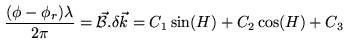
Once the baseline is fully calibrated (
![]() ) the exact source coordinates are known from the
) the exact source coordinates are known from the
![]() vector components. These components are formally deduced from
the differential of
vector components. These components are formally deduced from
the differential of
![]() . In the right-handed equatorial
system defined in Section 20.2 we obtain
. In the right-handed equatorial
system defined in Section 20.2 we obtain
| (20.9) | |||
 |
(20.10) |
| (20.11) | |||
| (20.12) | |||
| (20.13) |
Measurement of the phase at time intervals spanning a broad hour angle interval
allows us to determine the three unknowns ![]() ,
, ![]() , and
, and ![]() , and hence
, and hence
![]() and
and
![]() and the exact source position. Note that for sources close to the equator,
and the exact source position. Note that for sources close to the equator,
![]() and
and ![]() alone cannot accurately give
alone cannot accurately give
![]() . In the latter case,
. In the latter case, ![]() must be
determined in order to obtain
must be
determined in order to obtain
![]() ; this requires to accurately know the
instrumental phase and that the baseline is not strictly oriented along the E-W direction
(in which case there is no polar baseline component).
; this requires to accurately know the
instrumental phase and that the baseline is not strictly oriented along the E-W direction
(in which case there is no polar baseline component).
A synthesis array with several, well calibrated, baseline orientations is thus a
powerful instrument to determine
![]() . In practice, a least-squares analysis
is used to derive the unknowns
. In practice, a least-squares analysis
is used to derive the unknowns
![]() and
and
![]() from the measurements of
many observed phases
from the measurements of
many observed phases ![]() (at hour angle
(at hour angle ![]() ) relative to the expected phase
) relative to the expected phase
![]() . This is obtained by minimizing the quantity
. This is obtained by minimizing the quantity
![]() with respect to
with respect to ![]() ,
, ![]() , and
, and ![]() where
where
![]() . A complete analysis should give the
variance of the derived quantities
. A complete analysis should give the
variance of the derived quantities
![]() and
and
![]() as well as the
correlation coefficient.
as well as the
correlation coefficient.
Of course we could solve for the exact source coordinates and baseline components simultaneously. However, measuring the baseline components requires to observe several quasars widely separated on the sky. At mm wavelengths where atmospheric phase noise is dominant this is best done in a rather short observing session whereas the source position measurements of often weak sources are better determined with long hour angle coverage. This is why baseline calibration is usually made in separate sessions with mm-wave connected-element arrays.
The equation giving the source coordinates can be reformulated in a more compact
manner by using the components ![]() and
and ![]() of the baseline projected in a plane normal to
the reference direction. With
of the baseline projected in a plane normal to
the reference direction. With ![]() directed toward the north and
directed toward the north and ![]() toward the east, the
phase difference is given by
toward the east, the
phase difference is given by
| (20.14) |
| (20.15) | |||
| (20.16) |
| (20.17) |
| (20.18) | |||
In order to derive the unknowns
![]() and
and
![]() the least-squares
analysis of the phase data is now performed using the components
the least-squares
analysis of the phase data is now performed using the components ![]() derived at
hour angle
derived at
hour angle ![]() . In the interesting case where the phase noise of each phase sample is
constant (this occurs when the thermal noise dominates and when the atmospheric phase
noise is ``frozen'') one can show that the error in the coordinates takes a simple
form. For a single baseline and for relatively high declination sources the position error
is approximated by the equation
. In the interesting case where the phase noise of each phase sample is
constant (this occurs when the thermal noise dominates and when the atmospheric phase
noise is ``frozen'') one can show that the error in the coordinates takes a simple
form. For a single baseline and for relatively high declination sources the position error
is approximated by the equation
| (20.19) |
We have shown that for a well calibrated interferometer the least-squares fit
analysis of the phase in the ![]() plane can give accurate source coordinates. However,
the exact source position could also be obtained in the Fourier transform plane by
searching for the coordinates of the maximum brightness temperature in the source map. The
results given by this method should of course be identical to those obtained in the
plane can give accurate source coordinates. However,
the exact source position could also be obtained in the Fourier transform plane by
searching for the coordinates of the maximum brightness temperature in the source map. The
results given by this method should of course be identical to those obtained in the
![]() plane although the sensitivity to the data noise can be different.
plane although the sensitivity to the data noise can be different.
Finally, it is interesting to remind that the polar component of the baseline does not appear in the equation of the fringe frequency which is deduced from the time derivative of the phase. There is thus less information in the fringe frequency than in the phase.