Let us start with two general and simple remarks. First, the phase equation in Section
20.2 or the least-square analysis of the ![]() data in Section 20.3 show
that higher position accuracy is achieved for smaller values of the fringe spacing
data in Section 20.3 show
that higher position accuracy is achieved for smaller values of the fringe spacing
![]() . Thus, for astrometry it is desirable to use long baselines and/or to go to
short wavelengths. However, the latter case implies that the phases are more difficult to
calibrate especially at mm wavelengths where the atmospheric phase fluctuations increase
with long baselines. Second, sensitivity is always important in radio astrometry. For a
point-like or compact source the sensitivity of the array varies directly as
. Thus, for astrometry it is desirable to use long baselines and/or to go to
short wavelengths. However, the latter case implies that the phases are more difficult to
calibrate especially at mm wavelengths where the atmospheric phase fluctuations increase
with long baselines. Second, sensitivity is always important in radio astrometry. For a
point-like or compact source the sensitivity of the array varies directly as
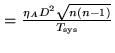
![]() where
where ![]() is the antenna diameter and
is the antenna diameter and ![]() the number of antennas. Thus, the
detection speed varies as
the number of antennas. Thus, the
detection speed varies as
![]() and big antennas are clearly advantageous
[Baudry 1996].
and big antennas are clearly advantageous
[Baudry 1996].
Comparison of the IRAM 5-element array with one of its competitors, the Owens Valley Radio
Observatory array (OVRO) with 6
![]() m, gives a ratio of detection speed of 1 over
0.36 at 3mm and 1 over 0.65 at 1.3mm in favour of the Plateau de Bure array (see Table
1 below where the two entries correspond to 3mm and 1mm; system temperatures have been
adopted according to advertised array specifications [June 2000]; sensitivity and speed
are defined in Table 1). (Note also that the sixth antenna in the Bure array will
increase its detection speed by 50%.) For comparison we include in Table 1 the BIMA
array located in California and the Nobeyama array in Japan (NMA). In addition, it is
interesting to note that the large dishes of the IRAM array are well adapted to quick
baseline and phase calibrations; this is another clear advantage of the IRAM
interferometer in astrometric observations.
m, gives a ratio of detection speed of 1 over
0.36 at 3mm and 1 over 0.65 at 1.3mm in favour of the Plateau de Bure array (see Table
1 below where the two entries correspond to 3mm and 1mm; system temperatures have been
adopted according to advertised array specifications [June 2000]; sensitivity and speed
are defined in Table 1). (Note also that the sixth antenna in the Bure array will
increase its detection speed by 50%.) For comparison we include in Table 1 the BIMA
array located in California and the Nobeyama array in Japan (NMA). In addition, it is
interesting to note that the large dishes of the IRAM array are well adapted to quick
baseline and phase calibrations; this is another clear advantage of the IRAM
interferometer in astrometric observations.
| BIMA | IRAM | NMA | OVRO | |||||
| Antennas | 9 | 5 | 6 | 6 | ||||
| Baseline (m) | 2000 | 400 | 400 | 480 | ||||
| Sensitivity | 0.31 | 0.26 | 1.00 | 1.00 | 0.42 | 0.06 | 0.36 | 0.65 |
| Speed | 0.10 | 0.07 | 1.00 | 1.00 | 0.18 | -- | 0.13 | 0.42 |
 ,
Speed
,
Speed
![$ =[\frac{\eta_AD^2\sqrt{n(n-1)}}{T_{\rm sys}}]^2$](img1941.png)
To illustrate the potential of the IRAM array for astrometry we consider here observations
of the SiO maser emission associated with evolved late-type stars. Strong maser line
sources are excited in the
![]() transition of SiO at 86 GHz and easily
observed with the sensitive IRAM array. Because of molecular energetic requirements (the
vibrational state
transition of SiO at 86 GHz and easily
observed with the sensitive IRAM array. Because of molecular energetic requirements (the
vibrational state ![]() lies some 2000 K above the ground-state) the SiO molecules must
not be located too much above the stellar photosphere. In addition, we know that the inner
layers of the shell expanding around the central star have sizes of order one arcsecond or
less. Therefore, sub-arcsecond position accuracy is required to locate the SiO sources
with respect to the underlying star whose apparent diameter is of order 20-50
milliarcseconds. For absolute position measurements one must primarily:
lies some 2000 K above the ground-state) the SiO molecules must
not be located too much above the stellar photosphere. In addition, we know that the inner
layers of the shell expanding around the central star have sizes of order one arcsecond or
less. Therefore, sub-arcsecond position accuracy is required to locate the SiO sources
with respect to the underlying star whose apparent diameter is of order 20-50
milliarcseconds. For absolute position measurements one must primarily:
Our first accurate radio position measurements of SiO masers in stars and Orion were
performed with the IRAM array in 1991/1992. We outline below some important features of
these observations [Baudry et al. 1994]. We used the longest E-W baseline available at that
time, about 300 m, thus achieving beams of order 1.5 to 2 arcseconds. The RF bandpass
calibrations were made accurately using strong quasars only. To monitor the variable
atmosphere above the array and to test the overall phase stability, we observed a minimum
of 2 to 3 nearby phase calibrators. Prior to the source position analysis we determined
accurate baseline components; for the longest baselines the r.m.s. uncertainties were in
the range 0.1 to 0.3 mm. The positions were obtained from least-square fits to the
imaginary part of the calibrated visibilities. (Note that the SiO sources being strong,
working in the ![]() or image planes is equivalent.)
or image planes is equivalent.)
The final position measurement accuracy must include all known sources of
uncertainties. We begin with the formal errors related to the data noise. This is due to
finite signal to noise ratio (depending of course on the source strength, the total
observing time and the general quality of the data); poorly calibrated instrumental phases
may also play a role. In our observations of 1991/1992 the formal errors were around 10 to
30 milliarcseconds. Secondly, phase errors arise in proportion with the baseline error
![]() and the offset between the unit vectors pointing toward the
stellar source and the nearby phase calibrator. This phase error is
and the offset between the unit vectors pointing toward the
stellar source and the nearby phase calibrator. This phase error is
![]() . Typical
values are
. Typical
values are
![]() mm and
mm and
![]() corresponding to phase errors of
corresponding to phase errors of ![]() to
to ![]() , that is to say less than the
typical baseline residual phases. A third type of error is introduced by the position
uncertainties of the calibrators. This is not important here because the accuracy of the
quasar coordinates used during the observations were at the level of one milliarcsecond.
, that is to say less than the
typical baseline residual phases. A third type of error is introduced by the position
uncertainties of the calibrators. This is not important here because the accuracy of the
quasar coordinates used during the observations were at the level of one milliarcsecond.
The quadratic addition of all known or measured errors is estimated to be around
![]() to
to ![]() . In fact, to be conservative in our estimate of the position accuracy
we measured the positions of nearby quasars using another quasar in the stellar field as
the phase calibrator. The position offsets were around
. In fact, to be conservative in our estimate of the position accuracy
we measured the positions of nearby quasars using another quasar in the stellar field as
the phase calibrator. The position offsets were around ![]() to
to ![]() depending on the
observed stellar fields; we adopted
depending on the
observed stellar fields; we adopted ![]() to
to ![]() as our final position accuracy of
SiO sources. The SiO source coordinates are derived with respect to baseline vectors
calibrated against distant quasars. They are thus determined in the quasi-inertial
reference frame formed by these quasars.
as our final position accuracy of
SiO sources. The SiO source coordinates are derived with respect to baseline vectors
calibrated against distant quasars. They are thus determined in the quasi-inertial
reference frame formed by these quasars.
Finally, it is interesting to remind a useful rule of thumb which one can use for
astrometry-type projects with any connected-element array provided that the baselines are
well calibrated and the instrumental phase is stable. The position accuracy we may expect
from a radio interferometer is of the order of 1/10th of the synthesized beam (1/20th if
we are optimistic). This applies to millimeter-wave arrays when the atmospheric
fluctuations are well monitored and understood. With baseline lengths around 400 m the
IRAM array cannot provide position uncertainties much better than about
![]() at 86
GHz. Extensions to one kilometer would be necessary to obtain a significant progress; the
absolute position measurements could then be at the level of 50 milliarcseconds which is
the accuracy reached by the best optical meridian circles.
at 86
GHz. Extensions to one kilometer would be necessary to obtain a significant progress; the
absolute position measurements could then be at the level of 50 milliarcseconds which is
the accuracy reached by the best optical meridian circles.
We have measured with the IRAM array the absolute position of the SiO emission sources associated with each spectral channel across the entire SiO emission profile. Any spatial structure related to the profile implies different position offsets in the direction of the star. Such a structure with total extent of about 50 milliarcseconds is observed in several late-type stars. This is confirmed by recent VLBI observations of SiO emission in a few stars. VLBI offers very high spatial resolution but poor absolute position measurements in line observations.
The best way to map the relative spatial structure of the SiO emission is to use the phase of one reference feature to map all other features. This spectral self-calibration technique is accurate because all frequency-independent terms are cancelled out. The terms related to the baseline or instrumental phase uncertainties as well as uncalibrated atmospheric effects are similar for all spectral channels and cancel out in channel to channel phase differences. By making the difference
| (20.20) |
| (20.21) |
![\resizebox{8.5cm}{!}{\includegraphics[angle=0]{baudryfig1.eps}}](img1961.png)
|
The relative spot maps obtained with connected-element arrays do not give the detailed spatial extent of each individual channel. This would require a spatial resolution of about one milliarcsecond which can only be achieved with VLBI techniques. Note however that VLBI is sensitive to strong emission features while the IRAM array allows detection of very weak emission; thus the two techniques appear to be complementary.
With SiO spatial extents of about 50 milliarcseconds and absolute positions at the level of 0.1 arcsecond it is still difficult to locate the underlying star. We have thus attempted to obtain simultaneously the position of one strong SiO feature relative to the stellar photosphere and the relative positions of the SiO sources using the 1 and 3 mm receivers of the IRAM array. This new dual frequency self-calibration technique is still experimental but seems promising.