For direct detection (or additive) interferometry, as in the optical domain,
an interferometer measures on-source on the baseline
![]() :
:
After doing an on-off (also called the ``sky calibration''), Eq.21.1 becomes:
Where
![]() is the visibility of the astronomical source measured
on baseline
is the visibility of the astronomical source measured
on baseline
![]() of amplitude
of amplitude
![]() and phase
and phase
![]() .
.
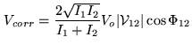
The visibility to calibrate can be expressed by:
![]() is the contrast which takes into account the calibration of all the system
(instrumentation + atmosphere). The photometric term is given by
is the contrast which takes into account the calibration of all the system
(instrumentation + atmosphere). The photometric term is given by
![]() (note that
(note that ![]() and
and ![]() are relatively easily measured).
are relatively easily measured).
The visibility
![]() appears as a fringe contrast (which is flux calibrated), therefore
it is normalized to unity. Note finally that in the optical case
appears as a fringe contrast (which is flux calibrated), therefore
it is normalized to unity. Note finally that in the optical case
![]() .
.
For heterodyne or multiplicative detection, the output of
the interferometer (correlator) gives a correlation rate ![]() which is a dimension less number (this uses a simple correlation
between two antennas, not a ``bi-spectrum'').
which is a dimension less number (this uses a simple correlation
between two antennas, not a ``bi-spectrum'').
The correlation corresponding to
![]() is the term of
astronomical interest, and is related to
is the term of
astronomical interest, and is related to ![]() by:
by:
At mm waves,
![]() because the atmospheric thermal
emission strongly dominates with typically
because the atmospheric thermal
emission strongly dominates with typically
![]() (except for the Sun and bright planets).
Therefore, Eq.21.3 simplifies as:
(except for the Sun and bright planets).
Therefore, Eq.21.3 simplifies as:
The heterodyne technique does not allow to measure the continuum term but preserves
the phase (thanks to the use of a complex correlator, see Chapter
2). ![]() can be seen as the correlation efficiency of the
interferometer (instrumental + atmospheric). The calibrated visibilities (as defined
in previous chapters)
can be seen as the correlation efficiency of the
interferometer (instrumental + atmospheric). The calibrated visibilities (as defined
in previous chapters)
![]() are expressed in unit
of flux density (Jy) while
are expressed in unit
of flux density (Jy) while
![]() can by considered as the photometric
term (including the photometric calibration of the atmosphere).
can by considered as the photometric
term (including the photometric calibration of the atmosphere).