


Next: 4.6 Conclusion
Up: 4. Introduction to Optical/Near-Infrared
Previous: 4.4 Formation of the
Contents
Subsections
4.5 Main challenges in interferometry
In this section, I address the main difficulties encountered in
optical interferometry. The main one is the effect of turbulence due
to the atmosphere. I will also tackle the limitation in terms of
performance due to the various types of noise.
4.5.1 Atmosphere turbulence
Figure 4.12:
Effect of the atmosphere turbulence on the incoming wavefronts.
|
|
The main effect of the presence of the atmosphere is the corrugation of the
incoming wavefronts. Due to difference of temperature between the ground
and the upper layers of the atmosphere, convection occurs and creates
turbulent eddies. These eddies are characterized by different temperature
and therefore different refractive indices. They move up and down with
different spatial scales. When looking to objects through the atmosphere,
the light rays are deviated randomly, i.e. the plane incoming wavefront is
corrugated by different phase delays depending on the total optical
thickness of the atmosphere along the propagation path (see Fig. 4.12). In optical interferometry, this phenomenon called
seeing yield two main consequences:
- at each telescope pupil entrance, the local wavefront is
corrugated. One does not get diffraction-limited images of the object,
but seeing-limited ones. In short exposure images and for multi-mode
interferometers, the image is formed of various speckles (see left panel
of Fig. 4.13) and in long-exposure images its typical size
is given by the characteristic size of turbulent cells where the light is
coherent, i.e. several tenths of meters. In addition, these features
move with time at timescale of several milliseconds. In the case of
single-mode interferometers, the speckles are spatially filtered at the
entrance of the interferometer and are translated in fluctuations of the
light coupling. Therefore one has to correct from the photometric
fluctuations induced by the turbulence (see right part of Fig. 4.13 and Sect. 4.5.3).
Figure 4.13:
Effect of the turbulence of each aperture. Left: in
multi-mode beam combination, the image is formed of speckles with
fringes at different phases (GI2T, adapted from [Labeyrie 1978]). Right: in
single-mode beam combination, the wavefront corrugation is
translated into photometric fluctuations
(IONIC, [Berger et al. 2001]). Upper curve: raw interferometric
signal; center curves: photometric signals; lower curve:
photometry-corrected interferometric signal (see also Sect. 4.5.3)
![\includegraphics[width=0.7\hsize]{atmosturb}](img567.png)
.
|
- the atmosphere induces fluctuations of the optical path
differences for each baseline. The result is that the fringes are not
stable at a given optical delay but randomly move around the sidereal
position. It is impossible to calibrate the phase of the fringes and
their amplitude is also decreased due to smearing during the integration
time.
Figure 4.14:
Optical path fluctuations due to the turbulence. Left:
simulations of the fluctuations for two Unit Telescopes at the
VLTI with typical seeing parameters (in microns). Right: the power
spectrum of the fluctuations follows a Kolmogorov law with a
saturation at low frequency due to the outer scale.
|
|
The atmosphere decorrelates the phase between different points
of the incoming wavefronts both in space and in time. That is why we
usually present the turbulence as yielding coherence volumes inside
which the wavefront can be considered as a non-disturbed plane wave.
The geometric parameters of the coherence cell are called the Fried's
parameters:
- -
- the size of the cell,
 , typically
 cm at
cm at
 and
and
 m at
m at
 depending of the turbulence strength.
- -
- the coherence time,
 , typically
ms at
and
, typically
ms at
and
 ms at
.
ms at
.
The turbulence occurs at different spatial scales and a popular
model is the Kolmogorov model that represents the power spectrum
of the turbulence as a power law [Roddier 1981]. However the
turbulence at small spatial frequencies saturates, i.e. the size
of the largest eddies is limited. This limit,  is called the
outer scale of the turbulence and is important in interferometry
since we estimate its size to be of the order of
is called the
outer scale of the turbulence and is important in interferometry
since we estimate its size to be of the order of
 m, typical lengths of most interferometer baselines. If the
baseline is larger than the outer scale then the effect of
turbulence is less than predicted by the Kolmogorov model.
m, typical lengths of most interferometer baselines. If the
baseline is larger than the outer scale then the effect of
turbulence is less than predicted by the Kolmogorov model.
4.5.2 Other atmosphere systematics
Figure 4.15:
Effect of the atmosphere refraction. The object image at
each telescope entrance is in fact a small spectrum. However
there is no effects on the optical delay since the optical path for
the two beams in the atmosphere is the same at each wavelength
 and
and  ,
and, the resulting OPD does not depend on wavelength. Even if
,
and, the resulting OPD does not depend on wavelength. Even if
 , we have
  and
and  , and
, and
 .
.
|
|
Optical interferometers must also take into account the atmospheric
refraction and the longitudinal spectral dispersion.
The wavelength dependence of the air refractive index implies
wavelength-dependent refraction angles when the light enters the
atmosphere. The atmosphere acts like a prism and the images at
each aperture are spectrally dispersed. Single mode
interferometers spatially filter the incoming wavefront, that
means they select a part of the image. Therefore this refraction
effect decreases the coupling factor in the interferometer. The
larger the telescope size, the smaller the diffraction-limited
images: this effect begins to be important for large telescopes.
Atmospheric dispersion
correctors are classical devices made of two prisms that can rotate and
compensate the dispersion due to the atmosphere refraction.
The refraction induces chromatic arrival angle, but does it result in
chromatic OPD. Fig. 4.15 shows that even if the
optical paths are different for two different wavelengths, they are the
same for each aperture and the OPD remains zero for all wavelengths. The
refraction does not yield a chromatic OPD.
However, the optical delay due to the zenith angle of the observed
object has to be compensated by delay lines. If the delay lines
are located in vacuum the compensation matches exactly the
geometrical delay above the atmosphere, but if the optical delay
in performed in air, then the compensation is performed only for
one wavelength because of the chromatism of the air refractive
index
 . The resulting OPD given by a delay of the
delay line that matches the geometrical delay
. The resulting OPD given by a delay of the
delay line that matches the geometrical delay  at
at
 is then:
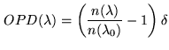 |
(4.5) |
Therefore the location of the zero-OPD changes with
wavelength. At high spectral resolution, the main effect is to twist
the fringes, whereas at low spectral dispersion the contrast of the
fringes can be severely decreased. To overcome this effect and besides using
vacuum delay lines, two translating prisms produce a variable glass
thickness that compensates exactly the chromatic OPD. This device
is called a longitudinal dispersion compensator.
4.5.3 Fighting the atmosphere: complexity and accuracy
The previous sections show that the propagation in the air implies
several problems. The chromatic effect of the air refractive index
can be compensated by an atmospheric dispersion compensator and a
longitudinal dispersion corrector. These phenomena are completely
predictable and therefore can easily be controlled by computer in
function of the zenith angle.
However the effect of the turbulence is much more difficult to control
since the time scale is of the order of several milliseconds and the
spatial scales are small. Adaptive optics (or tip-tilt compensation) and
fringe trackers are therefore required to increase the sensitivity of
optical interferometers (see Sect. 4.3). However
the correction is never perfect and some
residuals can still affect the signal.
One solution is to use speckle techniques to calibrate those
residuals. GI2T has proven that one can use several speckles to
calibrate the visibility of an object. Another method is to filter out
the incoming wavefront. The principle is well-known by the opticians:
they clean up images by placing so-called spatial
filters in the Fourier plane associated to the images. With a
pinhole at the focus of a telescope, the wavefront in the exit pupil
is then cleaned up and flat. The wavefront corrugation is transfered
in intensity fluctuations since the speckle image on the pinhole is not
stable. Optical waveguides, like optical fibers, are optical devices
that behave like infinitively small pinholes but with a high
coupling efficiency (typically 70%). The signal that exits from a
waveguide is an electric field whose shape is given by the geometry of
the waveguide (and therefore is fixed) and for which only two
parameters can vary: the global amplitude and the phase. By measuring the
variations for the photometry for each
beam, we can compute a visibility corrected from the
atmospheric perturbations. The visibility estimator,
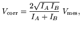 |
(4.6) |
little depends on the turbulence with
 the raw
visibility,
the raw
visibility,  and
and  the intensities measured for each beam.
Figure 4.16:
The FLUOR fiber beam combiner (right). Example of
incoming signals: left top panel shows the raw signal with two
photometry channels that monitors the coupling in the fibers;
left bottom panels shows the corrected interferogram
from [Coudé Du Foresto, Ridgway, & Mariotti 1997].
|
|
This method has proven to be very accurate in measuring
visibilities. FLUOR reaches 0.3% for some targets [Coudé Du Foresto, Ridgway, & Mariotti 1997].
However, one should keep in mind that the measured visibility is
not exactly the object visibility except if the objet is not
resolved by the individual apertures. When the object is larger
than the projected size of the spatial filter on the sky, one has
to apply a visibility correction using the information given by
the image obtained with the resolution of the individual
apertures.
4.5.4 Noise sources - Sensitivity
The signal measured with an optical interferometer is affected by
several sources of noises. In the case of the instrument AMBER on the
VLTI these sources of noises are:
Figure:
Signal-to-noise ratio computed for the AMBER instrument
at the VLTI in the K band (2.2
 ) for an object of visibility
of 1, a seeing of 0.5
) for an object of visibility
of 1, a seeing of 0.5 , a low dispersion, and a long exposure using
fringe tracking.
, a low dispersion, and a long exposure using
fringe tracking.
|
|
- -
- the photon noise is the fundamental noise associated to
the detection of the photons. It follows a Poisson-type statistics.
- -
- the detector read-out noise is the noise of the electronics
that reads the signal. It is an additive Gaussian noise with a
characteristic level called the read-out noise (RON).
- -
- the thermal noise is the noise that comes from the detection
of background photons. The background level is measured and
subtracted. The background estimation gives an error due to the
photon statistics.
- -
- the instrument OPD stability is not a noise that
affects the detected photons, but the measured visibility. The
residual motions of the optics in the instrument induce a blurring
of the fringes at a small level. In AMBER, we expect this level to
be lower than
 of the unit visibility.
- -
- the atmosphere fluctuations, even corrected by
simultaneous measurements of the photometry induce degradation of the
signal-to-noise ratio. The obvious situation is the case where no
photons are coupled into the interferometer.
Computing the error propagation in the final signal allows to calculate a
signal-to-noise ratio (SNR) for different type of situations. To illustrate
the consequence of the source brightness on the performance of an
interferometer, I show in Fig. 4.17 the SNR curve for
different star magnitudes in the case of the AMBER instrument on the unit
telescope of the VLTI with different typical values of the site.
For bright objects the dominant noise source is the instrument
stability. When observing faintest objects, the limitations become
first the photon noise, then depending on the integration time,
either the thermal background noise or the read-out noise.
Next: 4.6 Conclusion
Up: 4. Introduction to Optical/Near-Infrared
Previous: 4.4 Formation of the
Contents
Anne Dutrey
![\includegraphics[width=0.35\hsize]{piston2}](img568.png)
![\includegraphics[width=0.35\hsize]{piston1}](img569.png)
![\includegraphics[width=0.6\hsize]{refract}](img575.png)
![$\textstyle \parbox{0.4\hsize}{\centering
\includegraphics[width=\hsize]{fluor-uncor}\ *[1ex]
\includegraphics[width=\hsize]{fluor-cor}}$](img584.png)
![$\textstyle \parbox{0.55\hsize}{\includegraphics[width=\hsize]{fluor}}$](img585.png)
![\includegraphics[width=0.95\hsize]{amber-snr}](img586.png)
![\includegraphics[width=0.5\hsize]{wavefront_corrugation}](img566.png)