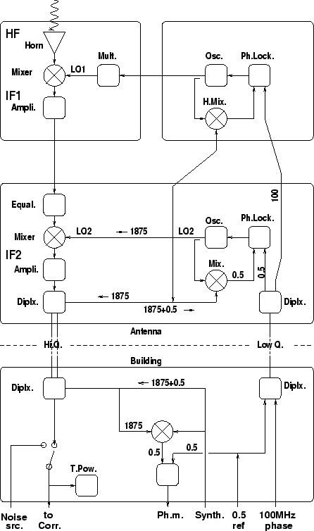
A block diagram of the Plateau de Bure interferometer system is shown in Fig. 7.3.
The signal path is outlined in Fig. 7.3. It shows the
signal and LO paths for one antenna and one receiver band. The high
frequency part (receiver) was described in Chapter 5. The
amplified first IF output (1275-1775 MHz) is down-converted to the
![]() MHz band and transported to the central building in a
high-quality cable. Before down-conversion, the band shape is
modified by a low-pass filter; since the LO2 is at a higher
frequency than the IF2, the bandpass will be reversed in the
conversion, and this by anticipation compensates for the frequency dependent
attenuation in the cable (which is of course higher at the high-frequency end of the
bandpass).
MHz band and transported to the central building in a
high-quality cable. Before down-conversion, the band shape is
modified by a low-pass filter; since the LO2 is at a higher
frequency than the IF2, the bandpass will be reversed in the
conversion, and this by anticipation compensates for the frequency dependent
attenuation in the cable (which is of course higher at the high-frequency end of the
bandpass).
The ![]() MHz band arriving in the central building is directed to
the correlator analog IF processor inputs (with a division by 6
since there are 6 identical correlator units) and to total power
detectors which are used for the atmospheric calibration and for the
radiometric phase correction.
MHz band arriving in the central building is directed to
the correlator analog IF processor inputs (with a division by 6
since there are 6 identical correlator units) and to total power
detectors which are used for the atmospheric calibration and for the
radiometric phase correction.
The first local oscillator is a Gunn oscillator (a tripler is used for
the 1.3mm receiver). The Gunn is phase-locked by mixing part of its
output with a harmonic of a reference signal (used also as the
second LO): the harmonic mixing produces a 100MHz signal, the phase
of which is compared to a reference signal at frequency
![]()
![]() MHz, coming from the
central building. That reference signal is used to carry the phase
commands to be applied to the first LO: a continuously varying phase
to compensate for earth motion and phase switching used to separate
the side-bands and suppress offsets.
MHz, coming from the
central building. That reference signal is used to carry the phase
commands to be applied to the first LO: a continuously varying phase
to compensate for earth motion and phase switching used to separate
the side-bands and suppress offsets.
The LO1 signal at
![]() may be locked either 100MHz above (``High
Lock'') or below (``Low Lock'') the
may be locked either 100MHz above (``High
Lock'') or below (``Low Lock'') the
![]() harmonic of the LO2
frequency
harmonic of the LO2
frequency
![]() :
:
| (7.17) |
The second local oscillator, at
![]() MHz, is
phase locked
MHz, is
phase locked
![]() =0.5 MHz below the frequency sent by the
synthesizer in the central building (which is under computer control and
common to all antennas):
=0.5 MHz below the frequency sent by the
synthesizer in the central building (which is under computer control and
common to all antennas):
| (7.18) |
The
![]() reference frequency is sent to all antennas from the
central building in a low quality cable, together with the
reference frequency is sent to all antennas from the
central building in a low quality cable, together with the
![]()
![]() MHz reference frequency for the first LO. The
MHz reference frequency for the first LO. The
![]() is
sent to the antennas via the same high-Q cable that transports the
IF2 signal.
No phase rotation is applied on the second local oscillator.
The relation between the RF signal frequencies (in the local rest
frame) in the upper and lower sidebands and the signal frequency in
the second IF band is thus (for high lock):
is
sent to the antennas via the same high-Q cable that transports the
IF2 signal.
No phase rotation is applied on the second local oscillator.
The relation between the RF signal frequencies (in the local rest
frame) in the upper and lower sidebands and the signal frequency in
the second IF band is thus (for high lock):
| (7.19) |
| (7.20) |
In each correlator a variable section of the IF2 band is down-converted to baseband by means of two frequency changes, with a fixed third LO (LO3) and a tunable fourth LO (LO4). It is on that LO4 that the phase rotations needed to compensate for residual phase drifts due to the geometrical delay change are applied (in fact that LO4 plays the role of the second frequency conversion in the above analysis). No phase rotation is applied on the second and third local oscillators.
The phase rotation applied on the fourth LO's is:
| (7.21) |
Short term phase errors in the local oscillators (jitter) will cause a decorrelation of the signal and reduce the visibility amplitude by a factor
| (7.22) |
|
|
0.99 | 0.98 | 0.95 | 0.90 |
| 5.75 | 8.1 | 13.0 | 18.5 |
The
![]() reference frequency is also used for a continuous control of
the electrical length of the High-Q cables transporting the IF2
signal from the antennas to the correlator room in the central building.
A variation
reference frequency is also used for a continuous control of
the electrical length of the High-Q cables transporting the IF2
signal from the antennas to the correlator room in the central building.
A variation ![]() in the electrical length of the High-Q cable
will affect the signal phase by
in the electrical length of the High-Q cable
will affect the signal phase by
![]() ; for a
length of 500m and a temperature coefficient of
; for a
length of 500m and a temperature coefficient of ![]() we have a
variation in length of 5mm or 17ps, which translates into a phase
shift of 4 degrees at the high end of the passband: this is a very
small effect.
we have a
variation in length of 5mm or 17ps, which translates into a phase
shift of 4 degrees at the high end of the passband: this is a very
small effect.
The same length variation induces a phase shift of
![]() degrees at the LO2 frequency. This signal being
multiplied by
degrees at the LO2 frequency. This signal being
multiplied by
![]() for the 1.3mm receiver, we have a totally unacceptable shift of
about 4 turns. The cables are buried in the ground for most of their
length; however they also run up the antennas and suffer from
varying torsions when the sources are tracked, and in particular when the
antenna is moved from the source to a phase calibrator.
for the 1.3mm receiver, we have a totally unacceptable shift of
about 4 turns. The cables are buried in the ground for most of their
length; however they also run up the antennas and suffer from
varying torsions when the sources are tracked, and in particular when the
antenna is moved from the source to a phase calibrator.
For this reason the electrical length of the cables is under permanent
control. The LO2 signal is sent back to the central building in the
High Q cable, and there it is mixed with the
![]() signal from the synthesizer. The phasemeter measures every second
the phase difference between the beat signal at 0.5 MHz and a
reference 0.5 MHz signal.
signal from the synthesizer. The phasemeter measures every second
the phase difference between the beat signal at 0.5 MHz and a
reference 0.5 MHz signal.
The measured phase difference is twice the phase offset affecting the
LO2, it is used by the computer to correct the LO1 phase
![]() after multiplication by
after multiplication by
![]() .
.