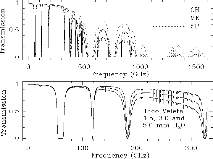
Calculations of zenith atmosphere opacity at 2.5 and 2.9 km, the
altitude of the IRAM sites, can be performed with the updated ATM
model [Pardo et al. 2001b] (see Figure 10.4). In fact, the
model itself has been installed on-line on the IRAM telescopes of
Pico Veleta and Plateau de Bure; it is activated at each
calibration or skydip and allows to interpret the observed sky
emissivity in terms of water and oxygen contributions and of upper
and lower sideband opacities. Note that the opacities derived from
sky emissivity observations do not always agree with those
calculated from the measurement of ![]() and the relative
humidity on the site, as water vapor is not at hydrostatic
equilibrium.
and the relative
humidity on the site, as water vapor is not at hydrostatic
equilibrium.
The typical zenith atmospheric opacities, in the dips of the 1.3 mm and 0.8 mm
windows (e.g. at the frequencies of the ![]() and
and ![]() rotational transitions of
CO, 230.54 and 345.80 GHz ), are respectively 0.15-0.2 and 0.5-0.7 in winter at the
IRAM sites. The
astronomical signals at these frequencies are attenuated by factors of respectively
rotational transitions of
CO, 230.54 and 345.80 GHz ), are respectively 0.15-0.2 and 0.5-0.7 in winter at the
IRAM sites. The
astronomical signals at these frequencies are attenuated by factors of respectively
![]() and 2 at zenith, 1.3 and 2.8 at 45 degree elevation, and 1.7 and 6 at
20 degree elevation. Larger attenuations are the rule in summer and in winter by
less favorable conditions. The
and 2 at zenith, 1.3 and 2.8 at 45 degree elevation, and 1.7 and 6 at
20 degree elevation. Larger attenuations are the rule in summer and in winter by
less favorable conditions. The ![]() line of CO, at 115.27 GHz, is close
to the 118.75 GHz oxygen line.
Although this latter is relatively narrow, it raises by
line of CO, at 115.27 GHz, is close
to the 118.75 GHz oxygen line.
Although this latter is relatively narrow, it raises by ![]() 0.3 the atmosphere
opacity (which is 0.35-0.4). The atmosphere attenuation is then intermediate
between those at 230 and 345 GHz (by dry weather, however, it is more stable than
the latter, since the water contribution is small). The measurement of accurate CO
line intensity ratios (even not considering the problems linked to differences in
beam size and receiver sideband gain ratios) requires therefore good weather, a high
source elevation, and a careful monitoring of the atmosphere.
0.3 the atmosphere
opacity (which is 0.35-0.4). The atmosphere attenuation is then intermediate
between those at 230 and 345 GHz (by dry weather, however, it is more stable than
the latter, since the water contribution is small). The measurement of accurate CO
line intensity ratios (even not considering the problems linked to differences in
beam size and receiver sideband gain ratios) requires therefore good weather, a high
source elevation, and a careful monitoring of the atmosphere.
During the past few years, new ground-based astronomical observatories have been built to allow access to the submillimeter range of the electromagnetic spectrum. Potential sites are now being tested for more ambitious instruments such as the Atacama Large Millimeter Array (ALMA). All of these are remote, high altitude sites. For our simulations we have selected three sites of interest for submillimeter astronomy: Mauna Kea, HI, USA (LAT=19:46:36, LONG=-155:28:18; home of the Caltech Submillimeter Observatory, James Clerk Maxwell Telescope and Submillimeter Array), Chajnantor, Chile (LAT=-23:06, LONG=-67:27; site selected for ALMA) and the Geographic South Pole (site of the Antarctic Submillimeter Telescope and Remote Observatory). The results of this comparison are also shown on Figure 10.4.
|
By analogy with the Rayleigh-Jeans approximation,
![]() , which strictly
applies to long wavelengths, the mm-wave radio astronomers have introduced the
concept of ``radiation'' or ``effective'' temperatures, which scale linearly
with the detected power.
, which strictly
applies to long wavelengths, the mm-wave radio astronomers have introduced the
concept of ``radiation'' or ``effective'' temperatures, which scale linearly
with the detected power.
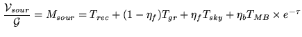
The noise power detected by the telescope is the sum of the power received by the
antenna,
![]() , and of the noise generated by the receiver and
transmission lines,
, and of the noise generated by the receiver and
transmission lines,
![]() .
.
Using Nyquist's relation
![]() ,
,
![]() and
and
![]() can be expressed in terms of the temperatures
can be expressed in terms of the temperatures ![]() and
and
![]() of two resistors, located at the end of the transmission line, which would
yield noise powers equal to
of two resistors, located at the end of the transmission line, which would
yield noise powers equal to
![]() and
and
![]() ,
respectively:
,
respectively:
![]() .
.
![]() is called the ``antenna temperature'' and
is called the ``antenna temperature'' and ![]() the ``receiver
temperature''.
the ``receiver
temperature''. ![]() becomes
becomes ![]() when the receiver horn sees a load, instead
of the antenna, and
when the receiver horn sees a load, instead
of the antenna, and ![]() when it sees the ground. It should be noted that
when it sees the ground. It should be noted that
![]() and
and ![]() are not stricto sensus equal to the load and ground physical
temperatures, but are only ``Rayleigh-Jeans'' equivalent of these temperatures (they
are proportional to the radiated power). For ambient loads, they approach
closely the physical temperature, since
are not stricto sensus equal to the load and ground physical
temperatures, but are only ``Rayleigh-Jeans'' equivalent of these temperatures (they
are proportional to the radiated power). For ambient loads, they approach
closely the physical temperature, since
![]() K at
K at
![]() mm.
mm.
When observing with the antenna a source and an adjacent
emission-free reference field, one sees a change
![]() in antenna temperature. Because of the
calibration method explained below, it is customary, in mm-wave
astronomy, to replace
in antenna temperature. Because of the
calibration method explained below, it is customary, in mm-wave
astronomy, to replace
![]() , the source antenna
temperature, by
, the source antenna
temperature, by
![]() , the source antenna temperature
corrected for atmosphere absorption and spillover losses. Both are
related through:
, the source antenna temperature
corrected for atmosphere absorption and spillover losses. Both are
related through:
![]() , where
, where ![]() is the line-of-sight
atmosphere opacity.
is the line-of-sight
atmosphere opacity. ![]() is the forward efficiency factor,
which denotes the fraction of the power radiated by the antenna on
the sky (typically of the order of 0.9, see also Chapter
1).
is the forward efficiency factor,
which denotes the fraction of the power radiated by the antenna on
the sky (typically of the order of 0.9, see also Chapter
1).
The source equivalent ``radiation temperature'' ![]() (often improperly called
``brightness temperature'' and therefore denoted
(often improperly called
``brightness temperature'' and therefore denoted ![]() when it is averaged over
the main beam) and
when it is averaged over
the main beam) and
![]() are related through
are related through
where
![]() is the antenna power pattern.
For a source smaller than the main beam,
is the antenna power pattern.
For a source smaller than the main beam,
![]() (where
(where ![]() is the beam efficiency
factor, see also Chapter 1).
is the beam efficiency
factor, see also Chapter 1).
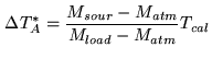
When observing a small astronomical source with temperature
![]() K, located at an elevation
K, located at an elevation ![]() , one
detects a signal
, one
detects a signal
![]() (of scale:
(of scale: ![]() volt or
counts per Kelvin):
volt or
counts per Kelvin):
This signal can be compared with the signals observed on the blank
sky (![]() ), close to the source, and to that observed on a hot load
(
), close to the source, and to that observed on a hot load
(![]() ):
):
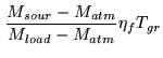
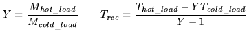
Let's assume that
![]() ;
then:
;
then:
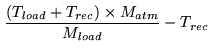
Typically, the mean atmosphere temperature is lower than the ambient temperature
near the ground by about 40 K:
![]() ; then, the
formula above still holds if we replace
; then, the
formula above still holds if we replace ![]() by:
by:
The receiver is not purely single-sideband. Let us denote by ![]() and
and ![]() the
normalized gains in the receiver lower and upper sidebands,
the
normalized gains in the receiver lower and upper sidebands,
![]() . The
atmosphere opacity per km varies with altitude as does the air temperature.
. The
atmosphere opacity per km varies with altitude as does the air temperature.
Then, the above expressions of ![]() and
and ![]() should be explicited for each
sideband (
should be explicited for each
sideband (![]() or
or ![]() ):
):