


Next: 11.6 Phase correction during
Up: 11. Atmospheric Fluctuations
Previous: 11.4 Remote sounding techniques
Contents
Remote sounding is done with the astronomical 1mm receivers in the inter-line region
at the chosen observing frequency. One uses the total power channel (bandwidth 500
MHz). Advantages of this approach are the close coincidence of observed and
monitored line of sight, and the fact that no additional monitoring equipment is
needed.
First success was on April 18, 1995, with the installation of the present receiver
generation on the PdBI [Bremer 1995]. Critical advantages were the improved total
power stability of the receivers and the capability to observe in the 1mm window.
The necessary stability for a
 phase rms at 230 GHz is about
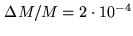 .
.
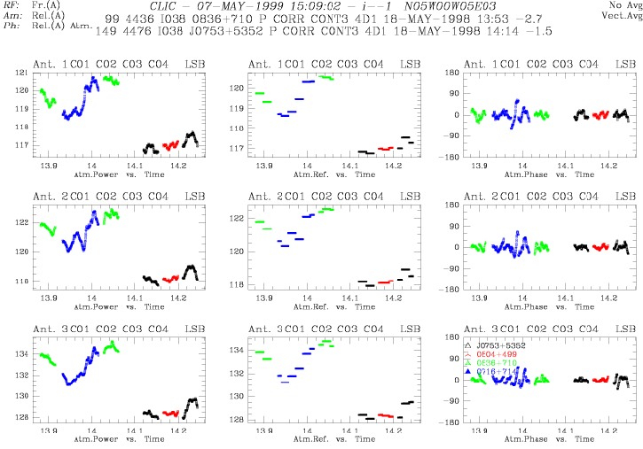
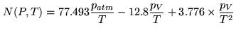
Figure 11.4:
Antenna based total power at 228.3 GHz, the reference value to calculate
the differential correction, and the model-based phase shift per antenna at
86.2 GHz.
 |
Steps of the method:
- Calibration of the total power counts
 to
to  as given in the lecture
on amplitude and flux calibration.
as given in the lecture
on amplitude and flux calibration.
- Iterate the amount of precipitable water vapor in an atmospheric model to reproduce
. There is no ``learning phase'' of the algorithm on a quasar, just the
model prediction.
- The amount of water vapor along the line of sight is proportional to the wet path
length.
 |
(11.13) |
However, wet path length and opacity have different dependencies on frequency,
atmospheric pressure and temperature which should be taken into account. The main
increase of the refractive index  of water vapor relative to dry air happens in
the infrared, which makes it difficult to use the Cramers-Kronig relations linking
it to opacity (integration over many transitions). For simplicity, we use the
calculations by [Hill & Cliffort 1981] for the frequency dependency and the temperature and
pressure dependencies by [Thayer 1974] instead. These references use not but
the refractivity
of water vapor relative to dry air happens in
the infrared, which makes it difficult to use the Cramers-Kronig relations linking
it to opacity (integration over many transitions). For simplicity, we use the
calculations by [Hill & Cliffort 1981] for the frequency dependency and the temperature and
pressure dependencies by [Thayer 1974] instead. These references use not but
the refractivity  , which is defined over the excess path length
  relative to
vacuum propagation over the line of sight
relative to
vacuum propagation over the line of sight  :
:
 |
(11.14) |
 |
(11.15) |
Hill and Cliffort calculate  for
for  K,
K,  mbar,
80% humidity
mbar,
80% humidity
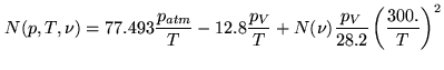 |
(11.16) |
- Subtract the average over a time interval (default: the duration of a scan) to
remove residual offsets due to receiver drift and ground pickup, which can be
different for each antenna (see Fig.11.4).
- Convert the antenna specific path shifts into phase at the observed wavelength,

- Calculate the baseline specific phase shifts
 . A corrected and an uncorrected version are calculated and
stored during the real time reduction which compresses the spectra over one scan.
The precision of the correction in relative pathlength is about
. A corrected and an uncorrected version are calculated and
stored during the real time reduction which compresses the spectra over one scan.
The precision of the correction in relative pathlength is about  m per antenna
(hence
m per antenna
(hence  m per baseline, i.e.
  larger).
- During the off-line data reduction, the user can choose freely between the corrected
and uncorrected sets. The phase correction can fail under the following conditions:
- Clouds:
the model only works for clear sky conditions, and will over-estimate the phase
shifts seriously in the presence of clouds.
- Very stable winter conditions:
The phase noise of the observations can be below
 at 230 GHz, which is the
intrinsic noise of the correction method.
at 230 GHz, which is the
intrinsic noise of the correction method.
- Total power instabilities:
For some frequencies, the receivers are difficult to tune. One can get a nice gain
in the interferometric amplitude, but an unstable total power signal with an
intrinsic noise well above at 230 GHz.
Even for the cases above, the observer has lost nothing because the uncorrected
scans are still there. Software tools are available which help to decide when to
apply the correction.
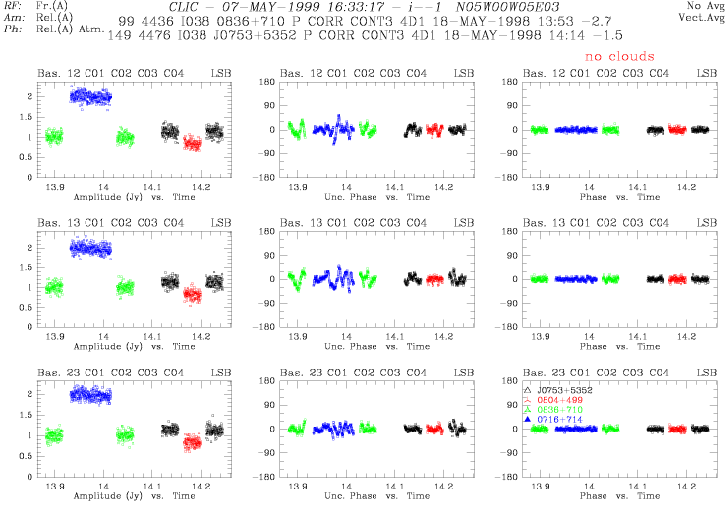
Figure 11.5:
Baseline based amplitudes, uncorrected phase and monitor corrected phase
at 86.2 GHz with a time resolution of 1 s. The data correspond to the antenna based
section in Fig.11.4. The phase calibration applied in columns 2 and 3 was
obtained using STORE PHASE /SELF on a one minute time scale, thereby
setting the mean phases to zero.
 |
Next: 11.6 Phase correction during
Up: 11. Atmospheric Fluctuations
Previous: 11.4 Remote sounding techniques
Contents
Anne Dutrey