After calibration with CLIC, the calibrated data may be stored in a
particular file called a `![]() table'. This is useful because much
of the data in the CLIC data file are not needed any more:
atmospheric parameters, total powers, image sideband visibilities,
data from other receivers may be discarded at this stage. All that
counts is: the data that are needed to describe the source itself,
the sky frequency that was observed, ... One may for instance create
a
table'. This is useful because much
of the data in the CLIC data file are not needed any more:
atmospheric parameters, total powers, image sideband visibilities,
data from other receivers may be discarded at this stage. All that
counts is: the data that are needed to describe the source itself,
the sky frequency that was observed, ... One may for instance create
a ![]() table for the continuum and one for each line that was
observed.
table for the continuum and one for each line that was
observed.
These ![]() tables are just special GILDAS tables suited for
tables are just special GILDAS tables suited for ![]() data
handling that are created by CLIC. Mapping consists of transforming
these tables into something more meaningful for the astronomer,
either images or numbers like positions, flux densities, sizes,
etc. However a good part of the data evaluation and analysis can be
directly performed on the
data
handling that are created by CLIC. Mapping consists of transforming
these tables into something more meaningful for the astronomer,
either images or numbers like positions, flux densities, sizes,
etc. However a good part of the data evaluation and analysis can be
directly performed on the ![]() data itself, before performing any of
the complex operations involved in creating an image (Fourier
transform and deconvolution). Direct analysis of the
data itself, before performing any of
the complex operations involved in creating an image (Fourier
transform and deconvolution). Direct analysis of the ![]() data is
the subject of this Lecture.
data is
the subject of this Lecture.
A ![]() table is a file in the Gildas Data Format, of dimensions
[3
table is a file in the Gildas Data Format, of dimensions
[3
![]() +7,
+7,
![]() ], for
], for
![]() spectral channels and
spectral channels and
![]() visibilities. The
visibilities. The
![]() lines contain:
lines contain:
The table header has the standard form of a GILDAS Image. The header is available (for instance) by declaring:
 GRAPHIC> SIC\DEFINE HEADER T co10.uvt READ
 GRAPHIC> EXAMINE T%
For a table named co10.uvt. Some keywords convey a more precise meaning for
GRAPHIC> HEADER co10.uvt
A set of commands to create a ![]() table may look like:
table may look like:
! Reset the default options:
  SET DEFAULT
! find the useful scans:
  FILE IN 21-JAN-1998-H126
  SET SOURCE IRC+10216
  SET RECEIVER 1
  SET PROCEDURE CORRELATION
  SET QUALITY AVERAGE
  FIND
! calibration options:
  SET AMPLITUDE ANTENNA RELATIVE
  SET PHASE ANTENNA RELATIVE INTERNAL ATMOSPHERE
  SET RF ANTENNA ON
! table creation:
  SET SELECTION LINE LSB L01
  TABLE HCN NEW /FREQUENCY HCN  88631.85 /RESAMPLE 19 10 -27 2.12 V
All but the last two commands should be familiar at this point.
If the data is spread on several files, one may go on by opening the other files, finding the data scans, and appending to the table:
  FILE IN 12-FEB-1998-H126
  FIND
  TABLE
  FILE IN 21-FEB-1998-H126
  FIND
  TABLE
...
(the arguments to TABLE need not to be repeated).
For continuum tables one may use:
SET SELECTION CONTINUUM DSB L01 TO L05 -
  /WINDOW 214405 214726 217476 217796 217837 217875
TABLE CONT-1MM NEW
Here we are using data from all the line subbands, but only in the three frequency windows: 214405 to 214726 MHz, 217476 to 217796MHz, and 217837 to 217875. This is of course to avoid the line emission of some molecules.
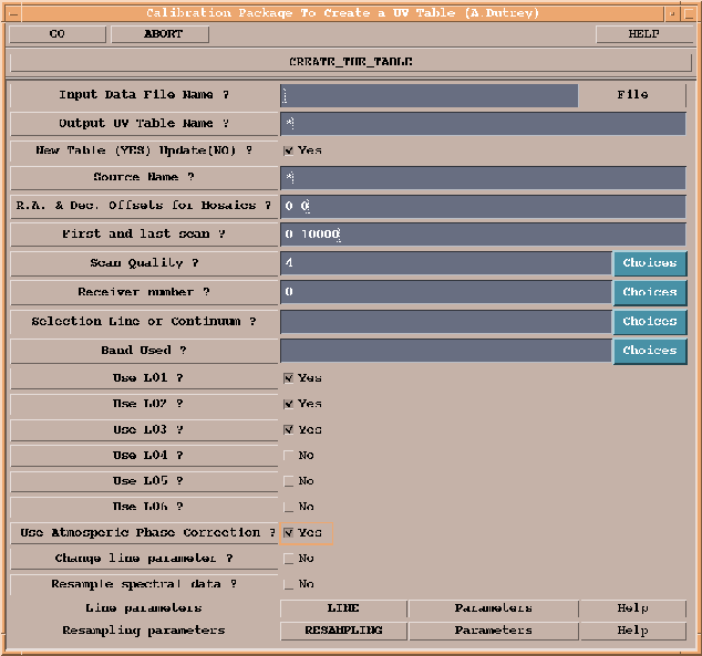
A standard menu is available under the CLIC main menu (``Create a UV Table''). After execution, a specific procedure is created to keep track of the options and parameters used. This procedure can subsequently be edited to add new data files (data files can also be added from the menu).