


Next: 14.3 Data editing
Up: 14. Plane Analysis
Previous: 14.1 tables
Contents
A procedure is available to do various plots from a continuum or line
table. Its name is UVALL and it is called by clicking on
``Interferometric UV operations'' in the GRAPHIC standard menu. One
has to select the first and last channel to be plotted (0 0 to get
all channels) and the name of the parameters to be plotted in
abscissa and ordinate. The following examples are the most useful
plots:
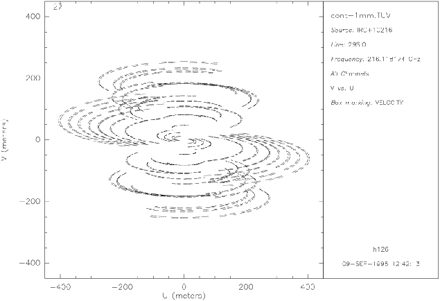
 coverage:
- to get an idea of the imaging quality that may
be obtained, to check if one configuration has been forgotten, ...
Figure 14.2:
Example of a
coverage plot
 |
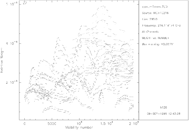
- weight vs. number:
- check if some data got strange weights
(e.g., zero) for any reason
Figure 14.3:
Weight versus
visibility number plot
 |
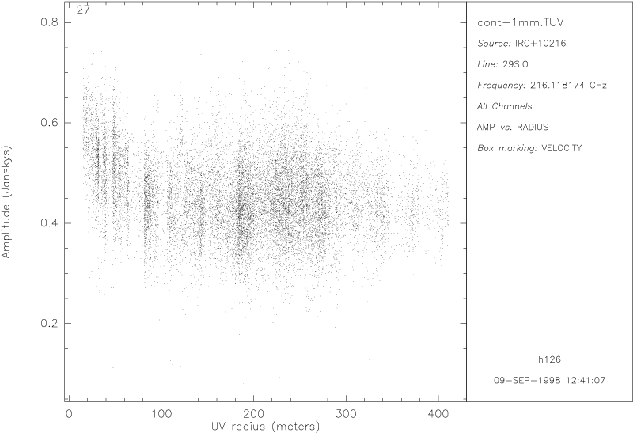
- Amplitude vs. antenna spacing:
- quite useful if a source is
strong to see if it looks resolved. Also check for spurious high
amplitude points.
Figure 14.4:
Amplitude
versus antenna spacing plot
 |
- Amplitude vs. weight:
- another useful check: spurious
high-amplitude points with non-negligible weight can cause a lot of
harm in a map.
These plotting facilities are also implemented in the MAPPING program
as a command (SHOW UV).
Next: 14.3 Data editing
Up: 14. Plane Analysis
Previous: 14.1 tables
Contents
Anne Dutrey