14.2 Object space

In the problems of Fourier synthesis encountered in astronomy, the object function of interest, $\Phi_{\! o}$, is a real-valued function of an angular position variable $\mathbf{\sigma} \equiv \mathbf{x} = (x,y)$. The geometrical elements under consideration are presented in Fig. 14.1.

  

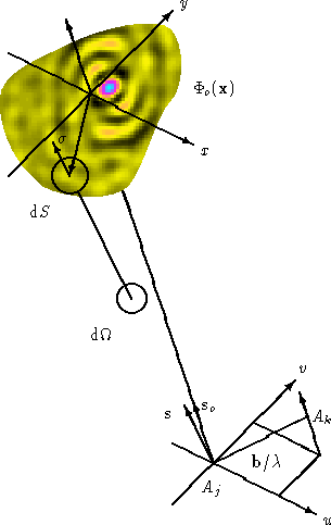
Figure: Traditional coordinate systems used to express the relation between the complex visibilities and the brightness distribution of a source under observation. Here, the two antennas A_j and A_kpoint toward a distant radio source in a direction indicated by the unit vector  s, and  b is the interferometer baseline vector. The position pointed by the unit vector  s_o is commonly referred to as the phase tracking center or phase reference position: $\mathbf{s} - \mathbf{s}_o = \mathbf{\sigma}$.

The object model variable $\phi$ lies in some object space H_o whose vectors, the functions $\phi$, are defined at a high level of resolution. This space is characterized by two key parameters: the extension $\Delta x$ of its field, and its resolution scale $\delta x$. To define this object space more explicitly, we first introduce the finite grid (see Fig. 14.2):

$$\text{\boldmath$G$\unboldmath } = \text{\boldmath$L$\unboldma... ...boldmath } : -\frac{N}{2} \leq p \leq \frac{N}{2}-1 \right\},$$ (14.1)

where N is some power of 2.

On each pixel $\mathbf{p}\,\delta x (\mathbf{p}\in\text{\boldmath$G$\unboldmath })$, we then center a scaling function of the form

$$e_{\mathbf{p}}(\mathbf{x}) = e_{\mathbf{0}}(\mathbf{x}-\mathb... ...}{\delta x}\bigr) \text{sinc} \bigl( \frac{y}{\delta x}\bigr).$$ (14.2)

  

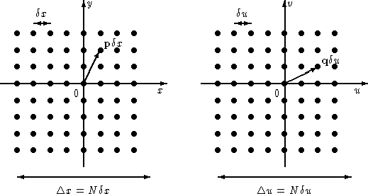
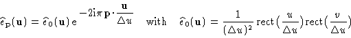
Figure: Object grid $\text{\boldmath $G$\unboldmath}\,\delta x$ (left hand) and Fourier grid $\text{\boldmath $G$\unboldmath}\,\delta u$ (right hand) for N=8. The object domain is characterized by its resolution scale $\delta x$and the extension of its field  $\Delta x = N\delta x$, where N is some power of 2 (the larger is N, the more oversampled is the object field). The basic Fourier sampling interval is  $\delta u = 1 / \Delta x$, the extension of the Fourier domain is  $\Delta u = 1/\delta x$.

It is easy to verify that these functions form an orthogonal set. In this presentation of WIPE, the object space H_ois the Euclidian space generated by the basis vectors e_p, p spanning $\text{\boldmath$G$\unboldmath }$ (see Fig. 14.2). The dimension of this space is equal to N²: the number of pixels in the grid  $\text{\boldmath$G$\unboldmath }$. The functions $\phi$ lying in H_o can therefore be expanded in the form

$$\phi(\mathbf{x}) = \sum_{\mathbf{p}\in\text{\boldmath$G$\unboldmath }} a_{\mathbf{p}} e_{\mathbf{p}}(\mathbf{x}),$$ (14.3)

where the  a_p's are the components of $\phi$ in the interpolation basis of H_o.

The Fourier transform of $\phi$ is defined by the relationship

   $$\widehat{\phi} (\mathbf{u}) = \int \phi(\mathbf{x}) \,\text{e... ...ext{i}\pi \mathbf{u}\!\cdot\!\mathbf{x}} \,\text{d}\mathbf{x},$$

where u is a two-dimensional angular spatial frequency: u = (u,v). According to the expansion of $\phi$ we therefore have:

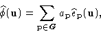$$\widehat{\phi} (\mathbf{u}) = \sum_{\mathbf{p}\in\text{\boldm... ...ldmath }} a_{\mathbf{p}} \widehat{e}_{\mathbf{p}}(\mathbf{u}),$$ (14.4)

where

$$\widehat{e}_{\mathbf{p}}(\mathbf{u}) = \widehat{e}_{\mathbf{0... ...c{u}{\Delta u}\bigr) \text{rect}\bigl(\frac{v}{\Delta u}\bigr)$$ (14.5)

and $\Delta u = 1/\delta x$.

The dual space of the object space, $\widehat{H}_o$, is the image of H_o by the Fourier transform operator: $\widehat{H}_o$ is the space of the Fourier transforms of the functions $\phi$ lying in H_o. This space is characterized by two key parameters: its extension  $\Delta u = 1/\delta x$, and the basic Fourier sampling interval  $\delta u = 1 / \Delta x$ (see Fig. 14.2).