12.4 Interferometric Calibration of the Amplitude

For antenna $i$, the antenna-based amplitude correction is given by (Eq.12.3 and 12.4).

$$a^K_i(t) = T^K_{cal_i}(t)G^{K}_i(\nu,t)\Gamma_i(t)$$ (12.14)

where K = U or L. The decorrelation factor $f$ (see Chapter 9) is not taken into account here because it is fundamentally a baseline-based parameter.

In a baseline-based decomposition, the complex gain of baseline $ij$, $\ensuremath{\mathcal{G}}_{ij}$ is given by:

$$\ensuremath{\mathcal{G}}^K_{ij}(t) = f \times a_i(t) a_j(t) e^{i(\phi_i(t)-\phi_j(t))}$$ (12.15)

and the amplitude of the baseline $ij$ is $\ensuremath{\mathcal{A}}_{ij}$

$$\ensuremath{\mathcal{A}}^K_{ij}(t) = f \sqrt{T^K_{cal_i}T^K_{cal_j}(t) G^{K}_i(\nu,t)G^{K}_j(\nu,t) \Gamma_i(t)\Gamma_j(t)}$$ (12.16)

We will discuss first the term $\Gamma_i$ and estimate then the decorrelation factor $f$, before giving a global scheme of the amplitude calibration.

12.4.1 Correction for the antenna gain $\Gamma _i(t)$

The antenna gain $\Gamma _i(t)$ corresponds to losses due to the antenna, mainly focus ($F_i$) and pointing ($P_i$) errors coming from thermal variations of the antenna structure and surface.

$$\Gamma_i(t) = P_i(t) \times F_i(t)$$ (12.17)

At Bure, we now check and correct automatically the pointing and the focus each hour. This correction is then done mainly in real time. This has improved a lot the quality of the data at 1.3mm. However, it is necessary in some cases to add a break in the amplitude (but not in the phase) fitting in order to take into account a focus error or a loss of amplitude due to pointing errors.

Note that an error on the focus of 0.1mm at 1.3mm will introduce a phase error of $\frac{4\pi}{\lambda}\times \frac{180}{\pi}\times 0.1 \sim 55^o$ and a loss in amplitude of $\sim 3-5\%$.

12.4.2 Estimate of the atmospheric decorrelation factor $f$

Details about the origin of $f$ are given in Chapter 11. I will discuss here the practical implementation of the atmospheric phase correction done in real-time and in CLIC. More details are given in the IRAM report ``Practical implementation of the atmospheric phase correction for the PdBI'' by R.Lucas.

The atmospheric phase fluctuations are due to different time varying water vapor content in the line-of-sight of each antenna through the atmosphere. Between antennas $i$ and $j$, this introduces a decorrelation factor $f\sim e^{-\Delta \phi^2_{ij}/2}$ on the visibility $V_{ij}$. This term, non-linear, cannot be factorized by antenna. Moreover due to the physical properties of the atmosphere, there are several timescales. One can correct partially some, but not all, of them.

At Bure the basic integration time is 1 second and the scan duration is usually 60 seconds. The radiometric correction works then on timescales of a few seconds to one minute. It corrects only the amplitude: the phase is never changed because phase jumps between individual scans are dominated by instrumental limitations (mainly the receiver stability on a few minutes + ground pickup variations). The implications on the image quality are developed in Chapter 18. Longer atmospheric timescales of about $2-8$ hours are removed by the spline functions fitted inside the phase and the amplitude.

Intermediate timescales fluctuations from about one minute (the scan duration) to 1 hour are not removed. The resulting rms phase are measured by the fit of the splines in the phase. These timescales are not suppressed by the radiometric correction, and they contribute to the decorrelation factor $f$ (see Eq.12.16), as the main component.

The decomposition of the atmospheric timescales for the PdBI observing method is given in table 12.3.

Table 12.3: Useful decomposition of the atmospheric phase fluctuations above the Plateau de Bure interferometer. This qualitative scheme is done to show which timescales are corrected by the calibration of the Bure data and the radiometric phase correction working at Bure.

Atmospheric Timescales	Amplitude coherence	Phase correction	Comments
$\Delta t \geq 1-2$ hours	No loss	Corrected	Large scales
		by temporal phase	are
		fitting	corrected
1 min $\leq \Delta t \leq 1-2$ hours	No correction	rms (= $\Delta \phi$) of	Loss of flux
1 min = scan duration		temporal phase fit
	can be	$f = e^{(-\Delta\phi^2/2)}$	a-posteriori correction by
	partially corrected	Radio Seeing	comparison with some
			reference sources: images
			of calibrators of known flux
$\Delta t \leq 1$ min	Usually corrected	``MONITOR 0'' $\equiv$	works usually well
	Radiometric phase	mean value of	except for
	correction	the phase in 1 min	bad weather conditions

12.4.2.0.1 The method

The differences in water vapor content are measurable by monitoring the variations of the sky emissivity $T_{sky}$. A monitoring of the total power in front of each antenna will then lead to a monitoring of the phase fluctuations. At Bure, we monitor the total power $M_{atm}$ with the 1.3mm receivers. The variation of $T_{sky}$, $\Delta T_{sky}$ (equal to $\Delta T_{emi}$) is linked to the total power by

$$\frac{\Delta M_{atm}}{M_{atm}} = \frac{(\Delta T_{emi} + \Delta T_{loss})}{T_{sys}}$$ (12.18)

The monitoring of the atmospheric phase fluctuation works only when $\Delta T_{loss}$ due to the instrumentation is negligible on the timescales at which the phase correction is calculated and applied (typically a few seconds to one minute). Slow drifts on scale of hours have no effects.

With standard atmospheric conditions and following [Thompson et al. 1986] (their Eq.13.20), the variation of the path length through the atmosphere at zenith can be approximated by:

$$\Delta L= 6.3 \delta w$$ (12.19)

were $\delta w$ is the variation of water vapor content. $\Delta L$ is related to the phase fluctuation $\psi_i$ above the antenna $i$ by

$$\psi_{i}(t) = \frac{2\pi}{\lambda}\Delta L(t)$$ (12.20)

For example, under standard conditions (see fig.12.1 or 12.2), a variation $\delta w =0.1$ mm corresponds to $\Delta L \simeq 630$ $\mu$m, $\Delta T_{sky}\simeq 1.5$ K and $\psi_i \simeq 250^o$ at 1.3mm. This value is enormous and would not allow to produce images of good quality.

To reduce the phase fluctuation to a reasonable value having a negligible impact on the image quality e.g. $\psi_i\sim 25^o$, one needs to get $\Delta T_{loss}+ \Delta T_{sky}\sim 0.15$ K corresponding to a global path length variation of $\sim 60 \mu m$. For a typical $T_{sys} \sim 150$ K (DSB in the antenna plane, not SSB outside the atmosphere as for astronomical use), the instrumental stability required ( $\Delta T_{loss} / T_{sys}$) must then be of order of $\sim 5 \cdot 10^{-4}$.

At Bure, on timescales of a few minutes, $\Delta T_{loss}$ is dominated by the stability of the receivers which must be carefully tuned to get the best stability. The 1.3mm receivers are systematically tuned to get a stability of a few $10^{-4}$; the stability is checked by doing autocorrelations of 60 seconds on the hot load. Achieving the required stability may prove impossible at some frequencies.

12.4.2.0.2 Practical implementation

Ideally one would like to use $T_{emi}$ measured each second on each antenna to compute $\psi_i(t)$ and correct the measured baseline phases. Practically, it is not so simple because $\psi_i(t)$ can do many turns and instrumental effects affect the measured $T_{emi}$.

Instead we use a differential procedure: once the antenna tracks a given source, one calibrates the atmosphere to calculate $T_{sys}(t_0)$, $\Delta L(t_0)$ and $\Delta L/d T_{sky}(t_0)$. Phase corrections are then referenced to $t_0$.

$$\Delta\psi_i = \frac{2\pi}{\lambda}\frac{d\Delta L}{d T_{emi}}\frac {T_{sys}(t_0)}{M_{atm}(t_0)}(M_{atm}(t)-M_{atm}(\mathrm{Ref}))$$ (12.21)

where $M_{atm}(\mathrm{Ref})$ is chosen in order to minimize as much as possible all the slow effects contributing to $\Delta T_{loss}$. A long term atmospheric effect can also be included in $M_{atm}(\mathrm{Ref})$ because these effects are not removed by the radiometric phase correction but by the traditional phase referencing on a nearby calibrator. The main steps are the following:

1. The total power $M_{atm}$ is continuously monitored on calibrators and on sources (every second).
2. Using the standard calibration method (see first part of the lecture) $M_{atm}$ and $T_{emi}$ (measured each second) are used to compute $T_{sky}$ and $w$.
3. The atmospheric model has also been upgraded to compute the path length $\Delta L$ and its derivative $d \Delta L/d T_{emi}$. $\Delta L$ is computed by integrating the refractive index of the wet air along the line of sight across the atmosphere.
4. Within the 60 seconds scan, the new phase (Eq.12.21) is computed and the correction applied to the amplitude.

12.4.2.0.3 Quasi-real Time Calibration

For the quasi-real time correction,

• the default value for $M_{atm}(\mathrm{Ref})$ is the measured atmospheric emission at the time of the last calibration, i.e. $M_{atm}(\mathrm{Ref})=M_{atm}(t_0)$.

12.4.2.0.4 Calibrating using CLIC

The CLIC command ``MONITOR $[delta-time]$'' allows to re-compute all the parameters. This command is useful when you want to select a better value for $M_{atm}(\mathrm{Ref})$.

• This command is used to prepare the atmospheric radiometric phase correction. It processes the calibration scans to compute the correction factors (i.e. the change of path length for a given change in emission temperature of the atmosphere at the atmospheric monitor frequency (normally 1.3mm)).

• The scans in the current index are grouped in intervals of maximum duration $[delta-time]$ (in seconds); source changes will also be used to separate intervals. In each interval a straight line is fitted in the variation of atmospheric emission as a function of time; this line will be the reference value for the atmospheric correction, i.e. the correction at time $t$ is proportional to the difference between the atmospheric emission at time $t$ and the reference at time $t$. This scheme is used to avoid contaminating the correction with total power drifts of non-atmospheric origin (changes in receiver noise and gain, and changes in ground noise).

• MONITOR 0 will use for each scan the average of the atmospheric emission as the reference value (i.e. $M_{atm}(\mathrm{Ref})=<M_{atm}(t)>_{scan}$). This will cause the correction to average to zero in one scan: the average phase is not changed, only the coherence is restored leading to an improved amplitude.

The automatic calibration procedure uses the command MONITOR 0.

Figure 12.5: The amplitude and phase versus time on baselines B12 and B13 with (histogram) and without (points) the radiometric phase correction. The phase remains unchanged but the amplitude is significantly improved.

12.4.3 Fitting Splines: the last step

In the real-time processing, only the receiver gain and bandpass, the atmospheric transmission and the radiometric correction have been calibrated.

Fitting of the temporal variations of the global antenna gain (the so-called amplitude calibration) is performed in CLIC by fitting splines functions with time steps of 3-6 hours (SOLVE AMPLITUDE [/WEIGHT] [/POL $degree$] [/BREAK $time$]) and can be done either in baseline-based or in antenna-based mode. Note that in the latter case, the averaged amplitude closures are computed, as well as their standard deviations. The amplitude closures should be close to 100%. Strong deviations of amplitude closures from 100% are an indication of amplitude loss on long baselines, due to phase decorrelation during the time averaging. The fit then shows systematic errors; if this occurs, baseline based calibration of the amplitudes might be preferred.

The amplitude calibration involves interpolating the time variations of the antenna gains measured with the amplitude calibrator, assuming the its flux is known. The fitted splines must be as smoothed as possible in order to minimize the errors introduced on the source which is observed in between calibrators.

12.4.4 A few final checks

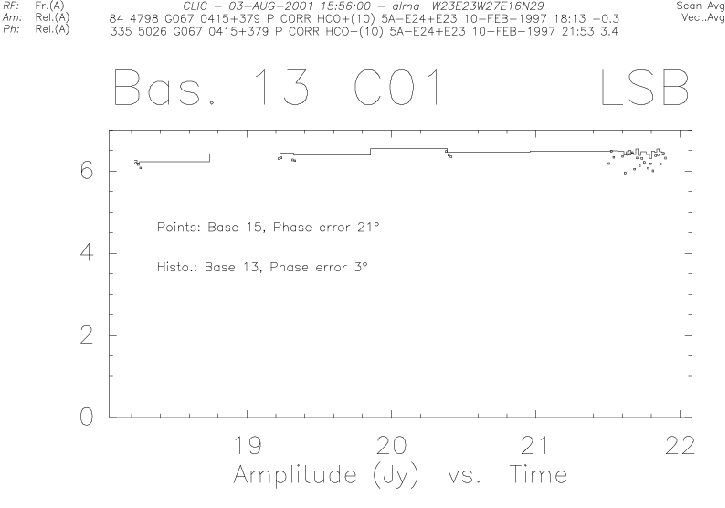
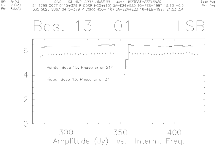
Once the amplitude calibration curve is stored, one can perform some simple checks on the calibrated data of the calibrator. These checks must be done in ${\rm Jy}$ (mode ``AMPLITUDE ABSOLUTE RELATIVE'' to the flux density of the calibrator).

Figure 12.6: Example of calibrated amplitude (Jy) versus time on a short (B13) and a long (B15) baseline. The amplitudes are similar.

12.4.4.0.1 Amplitude versus time

On each baseline, the amplitude curves should be flat and equal to assume the flux density of the calibrator.

12.4.4.0.2 Amplitude versus IF frequency

On each baseline, the amplitude curves should be flat, but they are not necessarily equal to flux of the calibrator because the decorrelation factor $f$ is not taken into account here. To retrieve the flux density of the calibrator, they must be multiplied by the corresponding $e^{-(\Delta \phi)^{2}/2}$, where $\Delta \phi$ is baseline rms phase noise determined during the phase calibration.

Figure 12.7: Example of calibrated amplitude versus IF frequency on a short (B13) and a long (B15) baseline. There is a significant loss of amplitude on the long baseline. The decorrelation factor is not calibrated out, and varies from short to long baselines. In this case, for the short baseline (B13), the decorrelation is completely negligible (see fig. 12.6).