


Next: 16.5 Implementation of WIPE
Up: 16. Advanced Imaging Methods:
Previous: 16.3 Experimental data space
Contents
Subsections
As the experimental frequency list is finite, and in
addition the experimental data blurred, the object
representation that can be obtained from these data is of
course incomplete. This simple remark shows that the inverse
problems of Fourier synthesis must be regularized: the
high-frequency components of the image to be reconstructed
must be negligible.
The central problem is to specify in which conditions it is possible
to extrapolate or interpolate, in some region of the Fourier domain,
the Fourier transform of a function  whose support is contained
in some finite region of
whose support is contained
in some finite region of  . It is now well established that
extrapolation is forbidden, and interpolation allowed to a certain extent.
The corresponding regularization principle is then intimately related to
the concept of resolution: the interpolation is performed in the frequency
gaps of the frequency coverage to be synthesized.
. It is now well established that
extrapolation is forbidden, and interpolation allowed to a certain extent.
The corresponding regularization principle is then intimately related to
the concept of resolution: the interpolation is performed in the frequency
gaps of the frequency coverage to be synthesized.
Let
 be the Fourier domain:
 . In Fourier synthesis, the frequency
coverage to be synthesized is a centro-symmetric
region
. In Fourier synthesis, the frequency
coverage to be synthesized is a centro-symmetric
region
 (see
Fig. 16.4).
(see
Fig. 16.4).
CLEAN and WIPE share a common objective, that of
the image to be reconstructed. This image,
 ,
is defined so that its Fourier transform is quadratically
negligible outside
,
is defined so that its Fourier transform is quadratically
negligible outside
 . More explicitly,
is defined by the convolution relation:
. More explicitly,
is defined by the convolution relation:
 |
(16.7) |
The ``synthetic beam''  is a function resulting from the
choice of
: the well-known clean beam
in CLEAN, the neat beam in WIPE.
is a function resulting from the
choice of
: the well-known clean beam
in CLEAN, the neat beam in WIPE.
The neat beam can be regarded as a sort of optimal
clean beam: the optimal apodized point-spread function
that can be designed within the limits of the Heisenberg
principle. More precisely, the neat beam is a
centro-symmetric function lying in the object
space , and satisfying the following properties:
- The energy of
 is concentrated in
.
In other words,
has to be small outside
in the mean-square sense: we impose the fraction
is concentrated in
.
In other words,
has to be small outside
in the mean-square sense: we impose the fraction  of this energy
in
to be close to
of this energy
in
to be close to  (say
(say
 ).
).
- The effective support
 of in is as small
as possible with respect to the choice of
and . The idea is of course to have the best possible
resolution.
of in is as small
as possible with respect to the choice of
and . The idea is of course to have the best possible
resolution.
This apodized point-spread function is thus computed on the grounds
of a trade-off between resolution and efficiency, with the aid of the
power method.
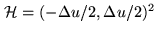
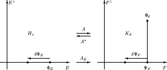
Figure:
Experimental frequency coverage and
frequency coverage to be synthesized
(left hand). The experimental frequency list
 includes
  frequency points. The
frequency coverage to be synthesized
is centred in the Fourier grid
frequency points. The
frequency coverage to be synthesized
is centred in the Fourier grid
 , where
 with
with  (here, the diameter of
the circle is equal to
(here, the diameter of
the circle is equal to
 ).
The neat beam (right hand) represented here
corresponds to the frequency coverage to be synthesized
for a given value of
).
The neat beam (right hand) represented here
corresponds to the frequency coverage to be synthesized
for a given value of
 . It is centred
in the object grid
. It is centred
in the object grid
 where
where
 (here, the full width of at half maximum is equal
to
(here, the full width of at half maximum is equal
to
 ).
).
![\begin{picture}(130,59)(0,0)
% width/height=435pt/400pt -> 63mm/58mm
\put(0,0){\...
...[width=60mm]{eafig4b.eps}}
\put(37,34){{\small$\mathcal{H}_s$}}
%%
\end{picture}](img1675.png) |
As extrapolation is forbidden, and interpolation only allowed to a
certain extent in the frequency gaps of the frequency coverage
to be synthesized, the experimental frequency list
should be completed by high-frequency points.
These points, located outside the frequency coverage to be
synthesized
, are those for which the high-frequency
components of the image to be reconstructed are practically
negligible.
The elements of the regularization frequency list
 are the frequency points
 located outside the
frequency coverage to be synthesized
at the nodes of the Fourier grid
:
located outside the
frequency coverage to be synthesized
at the nodes of the Fourier grid
:
 |
(16.8) |
The global frequency list
 is then the concatenation
of
with
.
is then the concatenation
of
with
.
According to the definition of the image to be reconstructed, the
Fourier data corresponding to
are defined by the relationship:
 |
(16.9) |
Clearly,
 lies in the experimental data space
  .
.
Let us now introduce the data vector:
 |
(16.10) |
This vector lies in the data space  , the real Euclidian space
underlying the space of complex-valued functions
, the real Euclidian space
underlying the space of complex-valued functions  on
,
such that
on
,
such that
 .
This space is equipped with the scalar product:
.
This space is equipped with the scalar product:
 |
(16.11) |
 is a given weighting function that
takes into account the reliability of the data via the standard
deviation
is a given weighting function that
takes into account the reliability of the data via the standard
deviation
 of
of
 , as well
as the local redundancy
, as well
as the local redundancy
 of
of
 up to
the sampling interval
up to
the sampling interval  .
.
The Fourier sampling operator  is the operator from
the object space into the data space :
is the operator from
the object space into the data space :
 |
(16.12) |
As the experimental data
are blurred values
of
 on
, this operator will
play a key role in the image reconstruction process. The definition of
this Fourier sampling operator suggests that the action of
should be decomposed into two components:
on
, this operator will
play a key role in the image reconstruction process. The definition of
this Fourier sampling operator suggests that the action of
should be decomposed into two components:  on the experimental
frequency list
, and
on the experimental
frequency list
, and  on the regularization
frequency list
.
on the regularization
frequency list
.
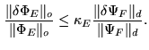
The reconstructed image is defined as the function  of the object space minimizing some objective functional.
The definition of this functional takes into account the nature of the
data, as well as other constraints. For example, the image to
be reconstructed may be confined to a subspace, or more generally
to a convex set, of the object space : this convex set
is the object representation space
of the object space minimizing some objective functional.
The definition of this functional takes into account the nature of the
data, as well as other constraints. For example, the image to
be reconstructed may be confined to a subspace, or more generally
to a convex set, of the object space : this convex set
is the object representation space  . It may be defined from
the outset (in an interactive manner, for example), or step by step
throughout the image reconstruction procedure (this is the case of
the current implementation of WIPE). In both cases, the projection
operator onto this space, the projector
. It may be defined from
the outset (in an interactive manner, for example), or step by step
throughout the image reconstruction procedure (this is the case of
the current implementation of WIPE). In both cases, the projection
operator onto this space, the projector  , will play an essential
role in the image reconstruction process.
, will play an essential
role in the image reconstruction process.
REMARK 1: positivity constraint.
In most cases encountered in practice, the scalar components of
in the interpolation basis of must be non-negative
(cf. Eq.![[*]](file:/usr/share/latex2html/icons/crossref.png) ).
In the current implementation of WIPE this constraint is taken
into account.
The object representation space is then built, step by step,
accordingly.
).
In the current implementation of WIPE this constraint is taken
into account.
The object representation space is then built, step by step,
accordingly.
The reconstructed image is defined as the function
minimizing on the objective functional:
 |
(16.13) |
According to the definition of the data vector
 and
to that of the Fourier sampling operator , this quantity
can be written in the form:
and
to that of the Fourier sampling operator , this quantity
can be written in the form:
 with with  |
(16.14) |
The experimental criterion  constraints the object
model to be consistent with the damped Fourier data
,
while the regularization criterion
constraints the object
model to be consistent with the damped Fourier data
,
while the regularization criterion  penalizes the high-frequency
components of .
penalizes the high-frequency
components of .
Let now  be the image of by (the space of the
  's,
spanning ),
's,
spanning ),  be the operator from into induced
by , and
be the operator from into induced
by , and  the projection of
onto (see Fig. 16.7).
The vectors minimizing
the projection of
onto (see Fig. 16.7).
The vectors minimizing  on , the solutions of the problem,
are such that
on , the solutions of the problem,
are such that
 . They are identical up to a vector
lying in the kernel of (by definition, the kernel of is the
space of vectors such that
. They are identical up to a vector
lying in the kernel of (by definition, the kernel of is the
space of vectors such that
 ).
).
As
 is orthogonal to , the solutions of the
problem are characterized by the property:
is orthogonal to , the solutions of the
problem are characterized by the property:
 .
On denoting by
.
On denoting by  the adjoint of , this property can also be
written in the form:
the adjoint of , this property can also be
written in the form:
 with with  |
(16.15) |
where  is regarded as a residue. This condition is of course equivalent
to
is regarded as a residue. This condition is of course equivalent
to  , where is the projector onto the object
representation space . The solutions of the problem are therefore
the solutions of the normal equation on :
, where is the projector onto the object
representation space . The solutions of the problem are therefore
the solutions of the normal equation on :
 |
(16.16) |
where
 .
.
Many different techniques can be used for solving the normal
equation (or minimizing on ). Some of these are certainly
more efficient than others, but this is not a crucial choice.
REMARK 2: beams and maps.
The action of  involved in
 is that of a
convolutor. As the two lists
and
are
disjoints, we have:
is that of a
convolutor. As the two lists
and
are
disjoints, we have:
 . Thus, the corresponding
point-spread function, called the dusty beam, has two components:
the traditional dirty beam
. Thus, the corresponding
point-spread function, called the dusty beam, has two components:
the traditional dirty beam  and the regularization
beam. The latter corresponds to the action of
and the regularization
beam. The latter corresponds to the action of  , the former
to that of
, the former
to that of  (see Fig. 16.5).
Likewise, according to the definition of the data vector,
(see Fig. 16.5).
Likewise, according to the definition of the data vector,
 is called the dusty map (as
opposed to the traditional dirty map
is called the dusty map (as
opposed to the traditional dirty map
 because
it is damped by the neat beam).
because
it is damped by the neat beam).
REMARK 3: construction of the object representation space.
With regard to the construction of the object
representation space , CLEAN and WIPE are
very similar: it is defined through the choice of the (discrete)
object support. It is important to note that this space may be
constructed, in a global manner or step by step, interactively or
automatically. In the last version of WIPE implemented at
IRAM, the image reconstruction process is initialized
with a few iterations of CLEAN. The support selected by
CLEAN is refined throughout the iterations of
WIPE by conducting a matching pursuit process at the
level of the components of in the interpolation basis
of : the current support is extended by adding the nodes of
the object grid
for which these
coefficients are the largest above a given threshold (half of the
maximum value, for example). The objective functional is then
minimized on that new support, and the global residue updated
accordingly. The object representation space of the
reconstructed image is thus obtained step by step in a
natural manner.
The simulation presented on Fig.16.5-16.6 corresponds
to the conditions of Fig. 16.4. The Fourier data
 were
blurred by adding a Gaussian noise:
for all
were
blurred by adding a Gaussian noise:
for all
 , the standard deviation
of
was set equal to
, the standard deviation
of
was set equal to  of the total
flux of the object (
of the total
flux of the object (
 ).
The image reconstruction process was initialized with a few
iterations of CLEAN, and the construction of the final
support of the reconstructed image was made as indicated
in Remark 3. At the end of the reconstruction process, a final
smoothing of the current object support was performed. In this
classical operation of mathematical morphology, the effective support
of ,
, is of course used as a structuring
element. The boundaries of the effective support of the reconstructed
neat map are thus defined at the appropriate resolution.
In particular, the connected entities of size smaller than that
of
are eliminated.
).
The image reconstruction process was initialized with a few
iterations of CLEAN, and the construction of the final
support of the reconstructed image was made as indicated
in Remark 3. At the end of the reconstruction process, a final
smoothing of the current object support was performed. In this
classical operation of mathematical morphology, the effective support
of ,
, is of course used as a structuring
element. The boundaries of the effective support of the reconstructed
neat map are thus defined at the appropriate resolution.
In particular, the connected entities of size smaller than that
of
are eliminated.
When the problem is well-posed, is a one-to-one map
(
 ) from onto ; the solution is then unique:
there exists only one vector
) from onto ; the solution is then unique:
there exists only one vector  such that
.
This vector, , is said to be the least-squares solution
of the equation
such that
.
This vector, , is said to be the least-squares solution
of the equation  ``=''
.
``=''
.
In this case, let
 be a variation of in ,
and
be a variation of in ,
and
 be the corresponding variation of in
(see Fig. 16.7).
It is easy to show that the robustness of the reconstruction process
is governed by the inequality:
be the corresponding variation of in
(see Fig. 16.7).
It is easy to show that the robustness of the reconstruction process
is governed by the inequality:
 |
(16.17) |
The error amplifier factor  is the condition number of :
 |
(16.18) |
here  and
and  respectively denote the smallest and the
largest eigenvalues of
.
The closer to is the condition number, the easier and the more robust
is the reconstruction process (see Fig. 16.8 and 16.9).
respectively denote the smallest and the
largest eigenvalues of
.
The closer to is the condition number, the easier and the more robust
is the reconstruction process (see Fig. 16.8 and 16.9).
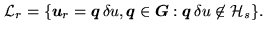
Figure 16.7:
Uniqueness of the solution and robustness of the
reconstruction process. Operator is an operator from the
object space into the data space .
The object representation space is a particular
subspace of . The image of by , the range of ,
is denoted by . In this representation, is the
projection of the data vector
onto . The inverse problem
must be stated so that is a one-to-one map from onto ,
the condition number having a reasonable value.
 |
The part played by inequality 16.17 in the development of the
corresponding error analysis shows that a good reconstruction
procedure must also provide, in particular, the condition
number . This is the case of the current implementation
of WIPE which uses the conjugate gradient method
for solving the normal equation 16.16.
To conduct the final error analysis, one is led to consider
the eigenvalue decomposition of
. This is done,
once again, with the aid of the conjugate gradient
method associated with the QR algorithm. At the cost
of some memory overhead (that of the  successive residues), the latter
also yields approximations of the eigenvalues
successive residues), the latter
also yields approximations of the eigenvalues  of
.
It is thus possible to obtain the scalar components of the associated
eigenmodes
of
.
It is thus possible to obtain the scalar components of the associated
eigenmodes  in the interpolation basis of .
The purpose of this analysis is to check whether some of them (in particular
those corresponding to the smallest eigenvalues) are excited or not
in . If so, the corresponding details may be artefacts of the
reconstruction.
in the interpolation basis of .
The purpose of this analysis is to check whether some of them (in particular
those corresponding to the smallest eigenvalues) are excited or not
in . If so, the corresponding details may be artefacts of the
reconstruction.
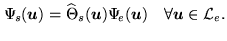
Figure:
Reconstructed neat map (left hand)
and eigenmode  (right hand) corresponding to the
smallest eigenvalue
(right hand) corresponding to the
smallest eigenvalue
 of
.
The conditions of the simulations are those of Fig. 16.4 and 16.5:
in particular,
the diameter of
is equal to
. The final condition
number is
of
.
The conditions of the simulations are those of Fig. 16.4 and 16.5:
in particular,
the diameter of
is equal to
. The final condition
number is
 (the eigenvalues of
are
plotted on the bar code below). This eigenmode is not excited in : the
separation angle
(the eigenvalues of
are
plotted on the bar code below). This eigenmode is not excited in : the
separation angle  between and is
greater than
between and is
greater than  . In other situations, when the final condition number
is greater, this mode may be at the origin of some artefacts in the
neat map (see Fig. 16.9).
. In other situations, when the final condition number
is greater, this mode may be at the origin of some artefacts in the
neat map (see Fig. 16.9).
![\begin{picture}(130,59)(0,0)
% width/height=388pt/378pt -> 60mm/59mm
\put(0,0){\...
...-> 60mm/59mm
\put(70,0){\includegraphics[width=60mm]{eafig8b.eps}}
\end{picture}](img1733.png)
|
The reconstructed map is then decomposed in the form:
 |
(16.19) |
The separation angle  between
and is explicitly given by the relationship:
between
and is explicitly given by the relationship:
 |
(16.20) |
The closer to  is , the less excited is the
corresponding eigenmode in the reconstructed
neat map .
is , the less excited is the
corresponding eigenmode in the reconstructed
neat map .
To illustrate in a concrete manner the interest of
equations 16.19 and 16.20, let us consider the
simulations presented in Fig. 16.4 and 16.9.
Whatever the value of the final condition number is, the error
analysis allows the astronomer to check if there exists a certain
similitude between some details in the neat map and some
features of the critical eigenmodes. This information is very
attractive, in particular when the resolution of the
reconstruction process is greater than a reasonable value (the
larger is the aperture to be synthesized
,
the smaller is the full width at half-maximum of ). In
such situations of ``super resolution,'' the error analysis will
suggest the astronomer to redefine the problem at a lower level of
resolution, or to keep in mind that some details in the
reconstructed neat map may be artefacts of the
reconstruction process.
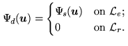
Figure:
Reconstructed neat map (left hand)
and related critical eigenmode (right hand). The latter
corresponds to the smallest eigenvalue
 of
.
The conditions of the simulations are those of Fig. 16.5, but here the diameter
of
is taken equal to
of
.
The conditions of the simulations are those of Fig. 16.5, but here the diameter
of
is taken equal to
 : the final condition number
is
: the final condition number
is
 (the eigenvalues of
are plotted
on the bar code below). The critical eigenmode is at the
origin of the oscillations along the main structuring entity of .
This mode is slightly excited (the separation angle
between and is less than
(the eigenvalues of
are plotted
on the bar code below). The critical eigenmode is at the
origin of the oscillations along the main structuring entity of .
This mode is slightly excited (the separation angle
between and is less than  ), thus the
corresponding details may be artefacts. In this case of ``super-resolution''
the error analysis provided by WIPE suggests that the procedure
should be restarted at a lower level of resolution (see Fig. 16.8),
so that the final solution be more stable and reliable.
), thus the
corresponding details may be artefacts. In this case of ``super-resolution''
the error analysis provided by WIPE suggests that the procedure
should be restarted at a lower level of resolution (see Fig. 16.8),
so that the final solution be more stable and reliable.
![\begin{picture}(130,59)(0,0)
% width/height=388pt/378pt -> 60mm/59mm
\put(0,0){\...
...-> 60mm/59mm
\put(70,0){\includegraphics[width=60mm]{eafig9b.eps}}
\end{picture}](img1743.png)
|
Next: 16.5 Implementation of WIPE
Up: 16. Advanced Imaging Methods:
Previous: 16.3 Experimental data space
Contents
Anne Dutrey
![\begin{picture}(130,59)(0,0)
% width/height=388pt/378pt -> 60mm/59mm
\put(0,0){\...
...-> 60mm/59mm
\put(70,0){\includegraphics[width=60mm]{eafig5b.eps}}
\end{picture}](img1720.png)
![\begin{picture}(130,59)(0,0)
% width/height=388pt/378pt -> 60mm/59mm
\put(0,0){\...
...-> 60mm/59mm
\put(70,0){\includegraphics[width=60mm]{eafig6b.eps}}
\end{picture}](img1721.png)