Some important mosaic properties can be understood by analyzing the
combination of the data directly in the ![]() plane. This analysis was
first proposed by [Ekers & Rots 1979]. The reader is also referred to
[Cornwell 1989]. We consider a source with a brightness distribution
plane. This analysis was
first proposed by [Ekers & Rots 1979]. The reader is also referred to
[Cornwell 1989]. We consider a source with a brightness distribution
![]() , where
, where ![]() and
and ![]() are two angular coordinates. The ``true''
visibility, i.e. the Fourier Transform of
are two angular coordinates. The ``true''
visibility, i.e. the Fourier Transform of ![]() , is noted
, is noted ![]() . An
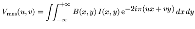
interferometer baseline, with two identical antennas whose primary
beam is
. An
interferometer baseline, with two identical antennas whose primary
beam is ![]() , measures a visibility at a point
, measures a visibility at a point ![]() which may
be written as:
which may
be written as:
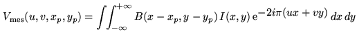
Now, let's imagine an ideal ``on-the-fly'' mosaic experiment: for a
given, fixed, ![]() point, the pointing direction is continuously
modified, and the variation of the visibility
point, the pointing direction is continuously
modified, and the variation of the visibility
![]() with
(
with
(![]() ,
, ![]() ) can thus be monitored. The Fourier Transform of these
data with respect to
) can thus be monitored. The Fourier Transform of these
data with respect to ![]() would give (from
Eq. 17.4):
would give (from
Eq. 17.4):
where:
For
![]() , we can thus derive:
, we can thus derive:
This relation illustrates an important property of the experiment we
have considered. The observations were performed at a given ![]() point but with a varying pointing direction.
Eq. 17.7 shows that is possible to derive from
this data set the visibility
point but with a varying pointing direction.
Eq. 17.7 shows that is possible to derive from
this data set the visibility
![]() at all
at all ![]() which
verify
which
verify
![]() . In other
terms, the measurements have been done at
. In other
terms, the measurements have been done at ![]() but the redundancy
of the observations allows to compute (through a Fourier Transform and
a division by the antenna transfer function) the source visibility at
all the points of a disk of radius
but the redundancy
of the observations allows to compute (through a Fourier Transform and
a division by the antenna transfer function) the source visibility at
all the points of a disk of radius
![]() , centered in
, centered in
![]() .
.
Interpretation
In very pictorial terms, one can say that the adjacent pointings
reinforce each other and thereby yield an estimate of the source
visibility at unmeasured points. Note however that the resulting
image quality is not going to be drastically increased: more
information can be extracted from the data, but a much more
extended region has now to be mapped17.2. The redundancy of
the observations has only allowed to rearrange the information in
the ![]() -plane. This is nevertheless extremely important, as e.g. it allows to estimate part of the missing short-spacings (see
below).
-plane. This is nevertheless extremely important, as e.g. it allows to estimate part of the missing short-spacings (see
below).
How is it possible to recover unmeasured spacings in the ![]() -plane?
It is actually obvious that two antennas of diameter
-plane?
It is actually obvious that two antennas of diameter ![]() ,
separated by a distance
,
separated by a distance ![]() , are sensitive to all the baselines
ranging from
, are sensitive to all the baselines
ranging from
![]() to
to
![]() . The measured
visibility is therefore an average of all these baselines:
. The measured
visibility is therefore an average of all these baselines:
![]() is actually the convolution of the ``true'' visibility by the
transfer function of the antennas. This is shown by the Fourier
Transform of Eq. 17.2, which gives:
is actually the convolution of the ``true'' visibility by the
transfer function of the antennas. This is shown by the Fourier
Transform of Eq. 17.2, which gives:
![]() . Now, if the pointing center and the phase center differ, a phase
gradient is introduced across the antenna apertures, which means that
the transfer function is affected by a phase term. Indeed, the Fourier
Transform of Eq. 17.3 yields:
. Now, if the pointing center and the phase center differ, a phase
gradient is introduced across the antenna apertures, which means that
the transfer function is affected by a phase term. Indeed, the Fourier
Transform of Eq. 17.3 yields:
| (17.8) |
Field spacing in a mosaic
In the above analysis, a continuous drift of the pointing direction
was considered. However, the same results can be reached in the case
of a limited number of pointings, provided that classical sampling
theorems are fulfilled. We want to compute the visibility in a finite
domain, which extends up to
![]() around the nominal
around the nominal
![]() point, and therefore the pointing centers have to be separated
by an angle of
point, and therefore the pointing centers have to be separated
by an angle of
![]() radians (see [Cornwell 1988]). In
practice, the (gaussian) transfer function of the millimeter dishes
drops so fast that one can use without consequences a slightly
broader, more convenient, sampling, equal to half the primary beam
width (i.e.
radians (see [Cornwell 1988]). In
practice, the (gaussian) transfer function of the millimeter dishes
drops so fast that one can use without consequences a slightly
broader, more convenient, sampling, equal to half the primary beam
width (i.e.
![]() ).
).
Mosaics and short-spacings
As with any other measured point in the ![]() plane, it is possible to
derive visibilities in a small region (a disk of diameter
plane, it is possible to
derive visibilities in a small region (a disk of diameter
![]() ) around the shortest measured baseline. This is the
meaning of the statement that mosaics can recover part of the
short-spacings information: a mosaic will include (
) around the shortest measured baseline. This is the
meaning of the statement that mosaics can recover part of the
short-spacings information: a mosaic will include (![]() ) points
corresponding to the shortest baseline minus
) points
corresponding to the shortest baseline minus
![]() .
.
In practice, however, things are more complex. First, we have to deal
with noisy data. As a consequence, it is not possible to expect a gain
of
![]() : the transfer function
: the transfer function ![]() which is used in
Eq. 17.7 is strongly decreasing, and thus
signal-to-noise ratio limits the gain in the
which is used in
Eq. 17.7 is strongly decreasing, and thus
signal-to-noise ratio limits the gain in the ![]() plane to a smaller
value, typically
plane to a smaller
value, typically
![]() ([Cornwell 1988]). This is still
a very useful gain: for the Plateau de Bure interferometer, this corresponds to a distance in
the
([Cornwell 1988]). This is still
a very useful gain: for the Plateau de Bure interferometer, this corresponds to a distance in
the ![]() plane of 7.5 m
plane of 7.5 m![]() , while the shortest (unprojected)
baseline is 24 m
, while the shortest (unprojected)
baseline is 24 m![]() . Secondly, the analysis described above
would be rather difficult to implement with real observations, which
have a limited number of pointing centers and different
. Secondly, the analysis described above
would be rather difficult to implement with real observations, which
have a limited number of pointing centers and different
![]() -coverages. Instead, one prefers to combine the observed fields
to directly reconstruct the sky brightness distribution. The resulting
image should include the information arising from the redundancy of
the adjacent fields, among them part of the short-spacings. However,
the complexity of the reconstruction and deconvolution algorithms that
have to be used precludes any detailed mathematical analysis of the
structures in the maps. For instance, the (unavoidable) deconvolution
of the image can also be interpreted as an interpolation process in
the
-coverages. Instead, one prefers to combine the observed fields
to directly reconstruct the sky brightness distribution. The resulting
image should include the information arising from the redundancy of
the adjacent fields, among them part of the short-spacings. However,
the complexity of the reconstruction and deconvolution algorithms that
have to be used precludes any detailed mathematical analysis of the
structures in the maps. For instance, the (unavoidable) deconvolution
of the image can also be interpreted as an interpolation process in
the ![]() plane (see
[Schwarz 1978] for the case of the CLEAN algorithm) and its effects
can thus hardly be distinguish from the intrinsic determination of
unmeasured visibilities that occur when mosaicing.
plane (see
[Schwarz 1978] for the case of the CLEAN algorithm) and its effects
can thus hardly be distinguish from the intrinsic determination of
unmeasured visibilities that occur when mosaicing.
}{T(u_p,v_p)}$](img1788.png)