


Next: 17.4 A CLEAN-based algorithm
Up: 17. Mosaicing
Previous: 17.2 Image formation in
Contents
Observation and calibration
The observation of a mosaic with the Plateau de Bure interferometer and the calibration of the
data do not present any specific difficulties. We just mention here a
few practical remarks:
- As shown in the previous paragraph, the optimal spacing between
adjacent fields is half the half-power primary beam width. Larger
separations can be used (e.g. to map larger field of view in the same
amount of time) but the image reconstruction is not optimal in that
case. Since observations are performed with dual-channel receivers
(operating at 1.3 and 3 mm), the field spacing has to be chosen for
one of the frequencies. Consequently, the mosaic observed at the other
frequency is either under- or oversampled.
- Even if this is not formally required by the reconstruction and
deconvolution algorithm described in the following section, it seems
quite important to ensure similar observing conditions for all the
pointing centers. Ideally, one wants the same noise level in each
field - so that the noise in the final image is uniform - and the
same
 -coverage - to avoid strong discrepancies (in terms of
angular resolution and image artifacts) between the different parts of
the mosaic. In practice, the fields are observed in a track-sharing
mode, i.e. in a loop with a few minutes integration time per pointing
direction: hence, atmospheric conditions and -coverage are similar
for all the fields.
-coverage - to avoid strong discrepancies (in terms of
angular resolution and image artifacts) between the different parts of
the mosaic. In practice, the fields are observed in a track-sharing
mode, i.e. in a loop with a few minutes integration time per pointing
direction: hence, atmospheric conditions and -coverage are similar
for all the fields.
- In most cases, a mosaic is not observed during an amount of time
significantly larger than normal projects. As the observing time is
shared between the different pointing centers, the sensitivity of each
individual field is thus smaller than what would have been achieved
with normal single-field observations. Note however that the
sensitivity is further increased in the mosaic, thanks to the strong
overlap between the adjacent fields (see below,
Fig. 17.1).
- The number of fields, and therefore the size of the mosaic, is limited
by the requirement to get good enough sensitivity and -coverage
for all the fields in a reasonable amount of observing time. The
current observing mode used at the Plateau de Bure limits the maximum
number of fields to about 20. Observing more fields is in principle
possible, but would require (much) more observing time and/or an other
approach (e.g. mosaic of several mosaics). Note that in any case, the
-coverage obtained for each field is sparse as compared to normal
synthesis observations. Finally, a potential practical limitation is
the disk and memory sizes of the computers, as mosaicing requires to
handle very large data cubes.
- The calibration of the data, including the atmospheric phase
correction, is strictly identical with any other observation performed
with the Plateau de Bure interferometer, as only the observations of the calibrators (quasars)
are used. At the end of the calibration process, a table and then
a dirty map are computed for each pointing center.
Mosaic reconstruction
The point is now to reconstruct a mosaic from the observations of each
field, in an optimal way in terms of signal-to-noise ratio. For the
time being, let's forget the effects of the convolution by the dirty
beam. Each field  can then be written:
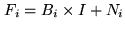 ,
where
,
where  is the primary beam of the interferometer, centered in a
different direction for each observation , and
is the primary beam of the interferometer, centered in a
different direction for each observation , and  is the
corresponding noise distribution. In practice, the same phase center
(i.e. the same coordinate system) is used for all the fields.
is the
corresponding noise distribution. In practice, the same phase center
(i.e. the same coordinate system) is used for all the fields.
Hence, the mosaic observations can be described as several
measurements of the same unknown quantity  , each one being
affected by a weighting factor . This is a classical
mathematical problem: the best estimate
, each one being
affected by a weighting factor . This is a classical
mathematical problem: the best estimate  of , in the
least-square sense, is given by:
of , in the
least-square sense, is given by:
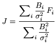 |
(17.9) |
where the sum includes all the observed fields and  is the rms of the noise distribution . (Note that in
Eq. 17.9 as well as in the following
equations, is a number while other letters denote
two-dimensional distributions).
is the rms of the noise distribution . (Note that in
Eq. 17.9 as well as in the following
equations, is a number while other letters denote
two-dimensional distributions).
Linear vs. non-linear mosaicing
The problem which remains to be address is the deconvolution of the
mosaic. This is actually the main difficulty of mosaic interferometric
observations. Two different approaches have been proposed
(e.g. [Cornwell 1993]):

- Linear mosaicing: each field is deconvolved
using classical techniques, and a mosaic is reconstructed afterwards
with the clean images, using Eq. 17.9.
- Non-linear mosaicing: a joint deconvolution of
all the fields is performed, i.e. the deconvolution is performed
after the mosaic reconstruction.
The deconvolution algorithms are highly non-linear, and the two
methods are therefore not equivalent. The first one is straightforward
to implement, but the non-linear mosaicing algorithms give much better
results. Indeed, the combination of the adjacent fields in a mosaic
allows to estimate visibilities which were not observed (see previous
paragraph), it allows to remove sidelobes in the whole mapped area,
and it increases the sensitivity in the (large) overlapping regions:
these effects make the deconvolution much more efficient.
Non-linear deconvolution methods based on the Maximum Entropy
Method (MEM) have been proposed by [Cornwell 1988] and
[Sault et al 1996]. As CLEAN deconvolutions are usually applied on
Plateau de Bure data, a CLEAN-based method adapted to the case of the
mosaics has been developed. The initial idea was proposed by
F. Viallefond (DEMIRM, Paris) and S. Guilloteau (IRAM), and the
algorithm is now implemented in the MAPPING software.
Next: 17.4 A CLEAN-based algorithm
Up: 17. Mosaicing
Previous: 17.2 Image formation in
Contents
Anne Dutrey