The behaviour of the mosaicing algorithm towards deconvolution
artifacts and/or instrumental effects can be studied by the means of
simulations of the whole mosaicing process. The simulations presented
below were computed with several models of sky brightness
distributions. ![]() -coverages of real observations were used
(4-antennas CD configuration of a source of declination
-coverages of real observations were used
(4-antennas CD configuration of a source of declination
![]() ). No noise has been added to the simulations shown in the
figures, so that pure instrumental effects can directly be seen.
). No noise has been added to the simulations shown in the
figures, so that pure instrumental effects can directly be seen.
 |
Stripes
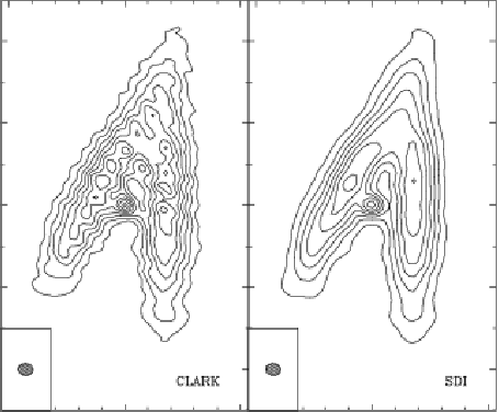
A well-known instability of the CLEAN algorithm is the formation of
stripes during the deconvolution of extended structures. After the
dirty beam has been subtracted from the peak of a broad feature, the
negative sidelobes of the beam are showing up as positive peaks. The
next iterations of the algorithm will then identify these artificial
peaks as CLEAN components. A regular separation between the CLEAN components is thereby introduced and the resulting map shows ripples
or stripes. [Steer et al. 1984] proposed an enhancement of CLEAN (implemented as the command SDI in MAPPING) which prevents such
coherent errors: the CLEAN components are identified and removed in
groups. As mosaics are precisely observed to map extended sources, the
formation of stripes can a priori be expected. Indeed, the
algorithm described in the previous paragraph presents this
instability. Fig. 17.2 shows an example of the
formation of such ripples. To make them appear so clearly, an
unrealistic loop gain (
![]() ) was used. Interestingly, the
algorithm of [Steer et al. 1984], adapted to the mosaics, does not result
in these stripes, even with the same loop gain. It seems thus to be a
very efficient solution to get rid of this problem, if it should
occur. Note however that more realistic simulations, including noise
and deconvolved with normal loop gain, do not show stripes
formation. This kind of artifacts seems thus not to play a significant
role in the image quality, for the noise and contrast range of typical
Plateau de Bure observations. In practice, they are never observed.
) was used. Interestingly, the
algorithm of [Steer et al. 1984], adapted to the mosaics, does not result
in these stripes, even with the same loop gain. It seems thus to be a
very efficient solution to get rid of this problem, if it should
occur. Note however that more realistic simulations, including noise
and deconvolved with normal loop gain, do not show stripes
formation. This kind of artifacts seems thus not to play a significant
role in the image quality, for the noise and contrast range of typical
Plateau de Bure observations. In practice, they are never observed.
Short-spacings
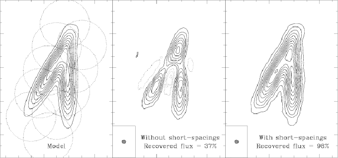 |
The mosaicing technique allows, at least in theory, to recover part of
the short-spacings information (see Section 17.2). In
practice, however, the lack of the short-spacings cannot be fully
compensated, and thus still introduces severe artifacts in the
reconstructed images. The mosaic case is actually more complex than
the single-field case, because the most extended structures are
filtered out in each field, thus introducing a lack of information on
an intermediate scale as compared to the size of the mosaic. As
a consequence, a very extended emission can be split into several
pieces, each one having roughly the size of the primary beam. This
effect can be very well seen on the simulation presented in
Fig. 17.3. To correct for this problem, it is
necessary to add the short-spacings informations (deduced typically
from single-dish observations) to the interferometric data set. Note
however that the effects of the missing short-spacings on the
reconstructed mosaic strongly depend on the actual ![]() -coverage of
the observations, as well as on the size and morphology of the source:
the artifacts can be small or negligible if the observed emission is
confined into reasonably small regions. From this point of view, the
example shown in Fig. 17.3 represents the worst
case.
-coverage of
the observations, as well as on the size and morphology of the source:
the artifacts can be small or negligible if the observed emission is
confined into reasonably small regions. From this point of view, the
example shown in Fig. 17.3 represents the worst
case.
In any case, CLEAN is known to be not optimal to deconvolve smooth, extended structures. In order to partially alleviate this problem and the effects of the missing short-spacings, [Wakker & Schwartz 1988] proposed an enhanced algorithm, the so-called multi-resolution CLEAN: deconvolutions are performed at low- and high-resolution, and the results are combined to reconstruct an image which then accounts for the extended structures much better than in the case of a classical CLEAN deconvolution. As already quoted before, this algorithm cannot be applied to a mosaic, because it relies on a linear measurement equation. A multi-resolution CLEAN adapted to mosaics has however been developed ([Gueth 1997]) and is implemented in MAPPING. This method will not be described here.
 |
Pointing errors
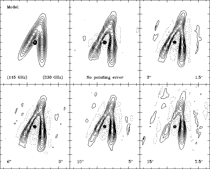
Pointing errors during the observations can of course strongly affect
the images obtained by mosaicing. The rms of the pointing errors of
the antennas of the Plateau de Bure interferometer is about ![]() . By comparison, the primary
beam size at 230 GHz is
. By comparison, the primary
beam size at 230 GHz is ![]() 22
22![]() (Table 17.1). The pointing errors are
difficult to model precisely: they are different for each antenna,
random errors as well as slow drifts occur, the amplitude calibration
partially corrects them, etc. A complete simulation should therefore
introduce pointing errors during the calculation of each
visibility. For typical Plateau de Bure observations, such a detailed modeling
is probably not necessary, as the final image quality is dominated by
deconvolution artifacts. To get a first guess of the influence of
pointing errors, less realistic simulations were thus performed, in
which each field is shifted as a whole by a (random) quantity. Such a
systematic effect most probably maximizes the distortions introduced
in the images. (Note that for a single field, the source would simply
be observed at a shifted position in such a simulation. For a mosaic,
the artifacts are different, because each individual field has a
different, random pointing error.
See [Cornwell 1987] for a simplified analysis in terms of
visibilities. Figure 17.4 presents typical
reconstructed mosaics for different rms of the pointing errors of
the Plateau de Bure antennas. Obviously, the larger the pointing error, the
worse the image quality. With a pointing error rms of
(Table 17.1). The pointing errors are
difficult to model precisely: they are different for each antenna,
random errors as well as slow drifts occur, the amplitude calibration
partially corrects them, etc. A complete simulation should therefore
introduce pointing errors during the calculation of each
visibility. For typical Plateau de Bure observations, such a detailed modeling
is probably not necessary, as the final image quality is dominated by
deconvolution artifacts. To get a first guess of the influence of
pointing errors, less realistic simulations were thus performed, in
which each field is shifted as a whole by a (random) quantity. Such a
systematic effect most probably maximizes the distortions introduced
in the images. (Note that for a single field, the source would simply
be observed at a shifted position in such a simulation. For a mosaic,
the artifacts are different, because each individual field has a
different, random pointing error.
See [Cornwell 1987] for a simplified analysis in terms of
visibilities. Figure 17.4 presents typical
reconstructed mosaics for different rms of the pointing errors of
the Plateau de Bure antennas. Obviously, the larger the pointing error, the
worse the image quality. With a pointing error rms of ![]() ,
reasonably correct mosaics can be reconstructed even at 230 GHz.
Clearly, care to the pointing accuracy has however to be exercised
when mosaicing at the highest frequencies.
,
reasonably correct mosaics can be reconstructed even at 230 GHz.
Clearly, care to the pointing accuracy has however to be exercised
when mosaicing at the highest frequencies.