


Next: 19.2 Spectral Line Sources
Up: 19. Low Signal-to-noise Analysis
Previous: 19. Low Signal-to-noise Analysis
Contents
Subsections
Let us start with a continuum source to simplify. The basic source parameters are
position (x,y), flux density S , and size. To determine the first 3 parameters,
the best strategy is to avoid resolving the source. Since the position errors are
proportional to the beam size, one should thus try to match the source size to the
beam size. Having a priori information on the source position (by other
observations, e.g. an optical image) will help to get a better accuracy on the
source flux.
, and size. To determine the first 3 parameters,
the best strategy is to avoid resolving the source. Since the position errors are
proportional to the beam size, one should thus try to match the source size to the
beam size. Having a priori information on the source position (by other
observations, e.g. an optical image) will help to get a better accuracy on the
source flux.
- Accurate Position: If the position is known to better than
1/10
 of the beam, you should then use UV_FIT with the
position fixed to determine the flux and the noise. In doing so, you should use an
appropriate fixed source size, based on any a priori information you have
(as you are following the ``best strategy'', this source size should be smaller than
the beam size). In such a case, you only have one free parameter, the flux, and a
of the beam, you should then use UV_FIT with the
position fixed to determine the flux and the noise. In doing so, you should use an
appropriate fixed source size, based on any a priori information you have
(as you are following the ``best strategy'', this source size should be smaller than
the beam size). In such a case, you only have one free parameter, the flux, and a  signal is sufficient to claim a detection.
- Rough Position If the source position accuracy is not sufficient,
you need to measure the position also. As you now have more parameters to derive, a
higher S/N will be required to do so. When the position uncertainty is about the
beam size, a 4
 signal will be required to get a firm detection. Use
UV_FIT to measure the flux and source position, with the same fixed source
size as before.
signal will be required to get a firm detection. Use
UV_FIT to measure the flux and source position, with the same fixed source
size as before.
- Unknown Position When the source position is really unknown, a 5
signal may become necessary to claim a detection. To locate the source position,
make an image first. Cleaning is usually not required at that level, unless the
sidelobe level is higher than the noise to signal ratio. Then, use UV_FIT to
measure the source flux, position and their associated errors, always using the same
fixed source size as before.
Note that in all cases, the source size being used should be at least equal to
the effective seeing of the observations, even if the source is actually a
point source.
Table 19.1 summarizes the procedure to be followed. Once you have done your
best in determining the source parameters, they remain to be properly interpreted.
As a rule of thumb, remember that All fluxes for detected weak sources are
biased by 1 to 2 . The only exception is when the source position and size
is known a priori. The reason for the bias is very intuitive. Assume you
have observed just enough to get a detection. A positive noise peak will
bring that up to a  value, a negative noise peak down to
  , which
you will consider as a non-detection.
, which
you will consider as a non-detection.
Table 19.1:
Recipes to use UV_FIT to measure the flux of a weak
source
| Rule 1 |
Do not resolve the source |
| Rule 2 |
Get the best absolute position before |
| Rule 3 |
Use UV_FIT to get |
| |
the parameters and their errors |
| |
a priori position accuracy |
| |
 Beam Beam |
 Beam Beam |
Any |
| Minimum signal |
3 |
4 |
5 |
| Position |
fixed |
free |
free, (make an image) |
| Source size |
fixed |
fixed |
fixed |
|
The other source parameters (position & size) require higher signal to noise to be
determined. The position accuracy is the synthesized beam size divided by the S/N
ratio. Hence, to get a position accuracy to 25 % of the beam size, at least a detection is required.
The above limitations are valid for a point source. If the source is not expected to
be small enough, additional complications occur. If you have performed the
experiment according to the guidelines given before (i.e. avoiding resolving the
source), the source size may be just about the beam size. In such circumstances, no
source size at all can be estimated with current mm interferometers if the detection
is less than  . To convince yourself, let us perform a simple thought
experiment. Assume we have detected a source at the level. Take this
signal, and divide the observations in two equal (in sensitivity) data
sets, one containing only the shortest baselines, the other ones only the longest
baselines. Each subset has a
. To convince yourself, let us perform a simple thought
experiment. Assume we have detected a source at the level. Take this
signal, and divide the observations in two equal (in sensitivity) data
sets, one containing only the shortest baselines, the other ones only the longest
baselines. Each subset has a  times higher noise level, and the error on
the flux difference between these two data sets is
times higher noise level, and the error on
the flux difference between these two data sets is  times the original noise
level. Assume that the shortest baselines give us twice more flux than the longest
one. In such a case, we would in fact have a better detection (
times the original noise
level. Assume that the shortest baselines give us twice more flux than the longest
one. In such a case, we would in fact have a better detection (
 ) with
the short baselines only, but the difference flux is only measured with
) with
the short baselines only, but the difference flux is only measured with
 . Such an experiment is not optimal from the detection point of view,
since we would have obtained a better result (
) by observing only half
of the time... Table 19.2 summarizes the corresponding numbers, and
indicates that the minimum detection level to resolve a source at the
. Such an experiment is not optimal from the detection point of view,
since we would have obtained a better result (
) by observing only half
of the time... Table 19.2 summarizes the corresponding numbers, and
indicates that the minimum detection level to resolve a source at the  level is
 .
.
Table 19.2:
Signal to Noise example for source size measurement. Line
(1) indicate the flux measured on short baselines, line (2) on long baselines, line
(3) the difference between (1) and (2), and line (4) the average. Three cases are
shown: a point source, a source with size similar to the beam, and the smallest
source which can be resolved at the level.
|
|
|
Point |
Beam Size |
Minimum Size |
|
|
|
Source |
Source |
Resolved |
|
|
|
Flux |
Noise |
S/N |
Flux |
Noise |
S/N |
Flux |
Noise |
S/N |
|
(1) |
Short baselines |
6 |
1.4 |
4.2 |
9 |
1.4 |
6.4 |
10 |
1.4 |
7.1 |
|
(2) |
Long baselines |
6 |
1.4 |
4.2 |
3 |
1.4 |
2.1 |
2 |
1.4 |
1.4 |
|
(3) |
Difference |
0 |
2 |
0 |
6 |
2 |
3 |
8 |
2 |
4 |
|
(4) |
Mean |
6 |
1 |
6 |
6 |
1 |
6 |
6 |
1 |
6 |
|
The interpretation of such data is made even more difficult by the fact that if the
size is unknown, the error on the total flux increases quite significantly.
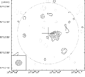
Fig.19.1 shows the detection of a weak high-redshift object in the Hubble
Deep Field area [Downes et al 1999]
Figure 19.1:
Left:  detection of the strongest source in the
Hubble Deep Field. Note that the contours are visually misleading (they start at 2
but with
detection of the strongest source in the
Hubble Deep Field. Note that the contours are visually misleading (they start at 2
but with  steps, given the impression of a much better
detection). Right: Attempt to derive a size. Size can be as large as the synthesized
beam... Note that the integrated flux increases with the source size.
steps, given the impression of a much better
detection). Right: Attempt to derive a size. Size can be as large as the synthesized
beam... Note that the integrated flux increases with the source size.
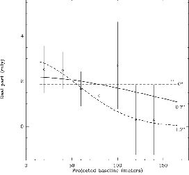 |
Although the detection is at the level, the source size is not
constrained by these observations, and the total flux becomes uncertain by as much
as 40 % when the uncertainty on the source size is included.
Next: 19.2 Spectral Line Sources
Up: 19. Low Signal-to-noise Analysis
Previous: 19. Low Signal-to-noise Analysis
Contents
Anne Dutrey