If the source position was a priori unknown, it is common practice to
determine it from the integrated line flux map made using the tailored line window
specified by the astronomer. Such a procedure results in a positively biased total
flux. Any speculated extension will also increase the total flux, by enlarging the
selected image region by selection of positive noise peaks. The net effect is a 1 to
2 ![]() positive bias on the integrated line flux. Things get really messy if a
continuum is superposed to the weak line...
positive bias on the integrated line flux. Things get really messy if a
continuum is superposed to the weak line...
A good strategy is required to minimize these biases. The correct approach to point
sources (or sources less than about
![]() of the synthesized beam), is
to first determine the position (e.g. from continuum data is available, or from the
integrated line map if not, or ideally from other data). Once the position is fixed,
the line profile can be derived by fitting a point (or small fixed size) source, at
fixed position into the
of the synthesized beam), is
to first determine the position (e.g. from continuum data is available, or from the
integrated line map if not, or ideally from other data). Once the position is fixed,
the line profile can be derived by fitting a point (or small fixed size) source, at
fixed position into the ![]() data. Using this line profile, the total line flux, as
well as source velocity and line width, can be derived by fitting an appropriate
lineshape, e.g. a Gaussian if no other information is available. In this last step,
a constant baseline offset should be added if there is a continuum contribution.
data. Using this line profile, the total line flux, as
well as source velocity and line width, can be derived by fitting an appropriate
lineshape, e.g. a Gaussian if no other information is available. In this last step,
a constant baseline offset should be added if there is a continuum contribution.
For extended sources, which may be affected by velocity gradient, one has to fit a
multi-parameter (6 for an elliptical gaussian) source model for each spectral
channel into the ![]() data. As a consequence, the signal in each channel should be
at least
data. As a consequence, the signal in each channel should be
at least ![]() to derive any meaningful information. The strict minimum is
to derive any meaningful information. The strict minimum is ![]() (per line channel...) to get flux and position for a fixed size source.
Velocity gradients are not believable unless even better signal to noise is obtained
per line channel !...Moreover, for narrow lines, most correlators produce
spectral channels which are not independent; the correlation between adjacent
channels should be taken into account when analyzing velocity gradients.
(per line channel...) to get flux and position for a fixed size source.
Velocity gradients are not believable unless even better signal to noise is obtained
per line channel !...Moreover, for narrow lines, most correlators produce
spectral channels which are not independent; the correlation between adjacent
channels should be taken into account when analyzing velocity gradients.
To sum up the weak spectral line problems:
Unfortunately, examples for such problems are numerous, especially for high redshift
CO lines. The ![]() galaxy 53W002 was detected in CO with the OVRO
interferometer by [Scoville et al 1997], who claim an extended source, with velocity
gradient. The published images (contour maps) look convincing, but this is biased by
the chosen visual representation, with contours starting at
galaxy 53W002 was detected in CO with the OVRO
interferometer by [Scoville et al 1997], who claim an extended source, with velocity
gradient. The published images (contour maps) look convincing, but this is biased by
the chosen visual representation, with contours starting at ![]() but spaced by
but spaced by
![]() . This creates the visual impression of higher S/N ratio. The published
spectra also looks convincing, but are presented as a fully sampled spectra (i.e.
channel width equal to twice the channel separation). Although this is the proper
way to present a complete information, the astronomer's eye is not accustomed to
such a presentation, and the astronomer tends to interpret the data as if the
channels were independent, thereby underestimating the noise. Yet the total line
flux is
. This creates the visual impression of higher S/N ratio. The published
spectra also looks convincing, but are presented as a fully sampled spectra (i.e.
channel width equal to twice the channel separation). Although this is the proper
way to present a complete information, the astronomer's eye is not accustomed to
such a presentation, and the astronomer tends to interpret the data as if the
channels were independent, thereby underestimating the noise. Yet the total line
flux is
![]() Jy.km/s i.e. (at best) only 7
Jy.km/s i.e. (at best) only 7 ![]() , and thus, according to
the discussion presented above, no extension/gradient should be measurable. Indeed,
using the IRAM interferometer, [Alloin et al 2000] find a line flux of
, and thus, according to
the discussion presented above, no extension/gradient should be measurable. Indeed,
using the IRAM interferometer, [Alloin et al 2000] find a line flux of
![]() Jy.km/s, no source extension, no velocity gradient, different line width and
redshift. Note that the line fluxes agree within the errors, with the second
determination just
Jy.km/s, no source extension, no velocity gradient, different line width and
redshift. Note that the line fluxes agree within the errors, with the second
determination just ![]() below the first one, as expected for an initially
biased result...
below the first one, as expected for an initially
biased result...
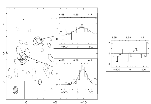
Another example of visually misleading result is shown in Fig.19.2. Although the two spectra appear different, there is a weak continuum (which was measured independently) on the Northern source. Once the continuum offset and a scale factor have been applied, the lack of visible structure in the difference spectrum shows that both line profiles are indistinguishable, i.e. that there is no measurable velocity gradient. These two sources could be lensed images of the same galaxy...
 |