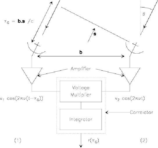
Figure 2.2 is a schematic illustration of a 2-antenna heterodyne interferometer.
The input (amplified) signals from 2 elements of the interferometer
are processed by a correlator, which is just a voltage multiplier followed
by a time integrator.
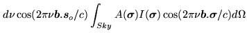
With one incident plane wave, the output ![]() is
is
As ![]() varies slowly because of Earth rotation,
varies slowly because of Earth rotation, ![]() oscillates as a cosine function, and is thus called the fringe pattern. As we had shown before that
oscillates as a cosine function, and is thus called the fringe pattern. As we had shown before that ![]() and
and ![]() were
proportional to the electric field of the incident wave, the
correlator output (fringe pattern) is thus proportional to the
power (intensity) of the wave.
were
proportional to the electric field of the incident wave, the
correlator output (fringe pattern) is thus proportional to the
power (intensity) of the wave.
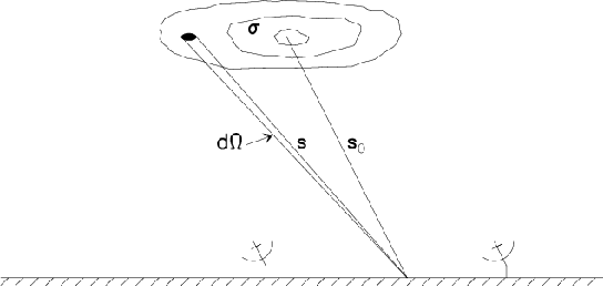
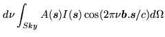
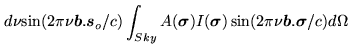
The signal power received from a sky area ![]() in direction
$s$ is (see Fig.2.3 for notations)
in direction
$s$ is (see Fig.2.3 for notations)
![]() over bandwidth
over bandwidth ![]() , where
, where
![]() is the
antenna power pattern (assumed identical for both elements, more
precisely
is the
antenna power pattern (assumed identical for both elements, more
precisely
![]() with
with ![]() the
voltage pattern of antenna
the
voltage pattern of antenna ![]() , and
, and
![]() is the sky
brightness distribution
is the sky
brightness distribution
 |
Two implicit assumptions have been made in deriving Eq.2.14. We assumed incident plane waves, which implies that the source must be in the far field of the interferometer. We used a linear superposition of the incident waves, which implies that the source must be spatially incoherent. These assumptions are quite valid for most astronomical sources, but may be violated under special circumstances. For example VLBI observations of solar system objects would violate the first assumption, while observations of celestial masers could violate the second one (if they were coherent as laboratory lasers, but observations have revealed astronomical masers are in fact incoherent).
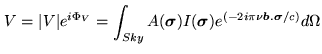
When the interferometer is tracking a source in direction
![]() , with
, with
![]()
We thus have
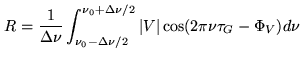
![$\displaystyle - \int_{-\Delta \nu /2}^{\Delta \nu / 2}
\vert V\vert \sin(2 \pi \nu_0 \tau_G- \Phi_V) \sin(2 \pi n \tau_g) dn ]$](img320.png)
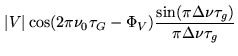
![$\displaystyle \frac{1}{\Delta \nu} \vert V\vert \cos( 2 \pi \nu_0 \tau_G- \Phi_...
... \pi n \tau_g) \right]_{-\Delta \nu /2}^{\Delta \nu / 2}
\frac{1}{2 \pi \tau_g}$](img321.png)
![$\displaystyle + \frac{1}{\Delta \nu} \vert V\vert \sin( 2 \pi \nu_0 \tau_G- \Ph...
... \pi n \tau_g) \right]_{-\Delta \nu /2}^{\Delta \nu / 2}
\frac{1}{2 \pi \tau_g}$](img322.png)