Next: 2.4 Fringe Stopping and
Up: 2. Millimetre Interferometers
Previous: 2.2 The Heterodyne Interferometer
Contents
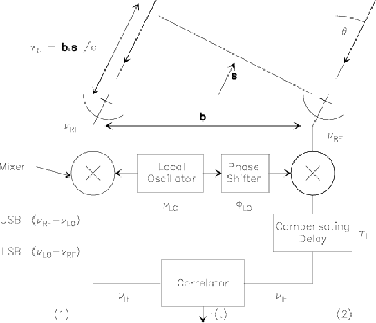
To compensate for the geometrical delay variations, delay lines
with mirrors (as in optics...) would be completely impractical
given the required size of the mirrors. The compensating delay is
thus performed electronically after one (or several) frequency
conversion(s), as illustrated in Fig.2.4. This can be
implemented either by switching cables with different lengths, or
in a more sophisticated way, by using shift memories after digital
sampling of the signal in the correlator. Apart for a few details
(see R.Lucas lecture, Chapter 7), the principle
remains identical.
In the case presented in Fig.2.4, for USB conversion, the phase changes of
the input signals from antenna 1 and 2 before reaching the correlator are
respectively
Introducing
 as the delay
tracking error, the correlator output is
as the delay
tracking error, the correlator output is
When the two sidebands are superposed, we can just sum the USB and LSB outputs,
which yields (after usual re-arrangement of the cosine expressions)
This shows that the amplitude is modulated by the delay tracking
error. The tolerance can be exceedingly small. For example, at
Plateau de Bure, the IF frequency  is 3 GHz, and a 1 %
loss is obtained as soon as the delay tracking error would be 7.5
picoseconds, i.e. a geometrical shift of 2.2 mm only. Due to Earth
rotation, the geometrical delay changes by such an amount in 0.1 s
for a 300 m baseline. Hence, delay tracking would have to be done
quite fast to avoid sensitivity losses. To avoid this problem, it
is common to use sideband separation. The delay tracking error
should then be kept small compared to the bandwidth of each
spectral channel,
is 3 GHz, and a 1 %
loss is obtained as soon as the delay tracking error would be 7.5
picoseconds, i.e. a geometrical shift of 2.2 mm only. Due to Earth
rotation, the geometrical delay changes by such an amount in 0.1 s
for a 300 m baseline. Hence, delay tracking would have to be done
quite fast to avoid sensitivity losses. To avoid this problem, it
is common to use sideband separation. The delay tracking error
should then be kept small compared to the bandwidth of each
spectral channel,
 , and the delay
can then be adjusted much less frequently.
, and the delay
can then be adjusted much less frequently.
Next: 2.4 Fringe Stopping and
Up: 2. Millimetre Interferometers
Previous: 2.2 The Heterodyne Interferometer
Contents
Anne Dutrey