Next: 2.6 Array Geometry &
Up: 2. Millimetre Interferometers
Previous: 2.4 Fringe Stopping and
Contents
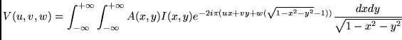
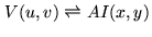
The Complex Visibility is
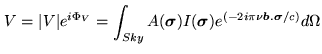 |
(2.31) |
Let  be the coordinate of the baseline vector, in units of the observing
wavelength
be the coordinate of the baseline vector, in units of the observing
wavelength  , in a frame of the delay tracking vector
 , with
  along
.
along
.  are the coordinates of the source vector
 in this frame.
Then
in this frame.
Then
Thus,
 |
(2.33) |
with
 when
when
 .
.
If  are sufficiently small, we can make the approximation
 |
(2.34) |
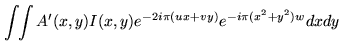
and Eq.2.33 becomes
i.e. basically a 2-D Fourier Transform of  , but with a phase error term
 . Hence, on limited field of views, the relationship between the sky
brightness (multiplied by the antenna power pattern) and the visibility reduces to a
simple 2-D Fourier transform.
. Hence, on limited field of views, the relationship between the sky
brightness (multiplied by the antenna power pattern) and the visibility reduces to a
simple 2-D Fourier transform.
There are other approximations related to field of view limitations. Let us
quantify these approximations.
- 2-D Fourier Transform
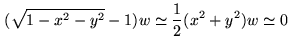
We can further neglect the phase error term in Eq.2.36, if the condition
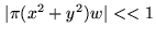 |
(2.37) |
is fulfilled. Now, note that
 |
(2.38) |
where
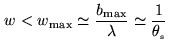
 is the synthesized beam width. Thus, if
 is the field of
view to be synthesized, the maximum phase error, obtained at the field edges
is the field of
view to be synthesized, the maximum phase error, obtained at the field edges
 , is
, is
 |
(2.39) |
Using
 radian (6
 ) as an upper limit (note that this
is the maximum phase error, i.e. the mean phase error is much smaller)
result in the condition (with all angles in radian...):
) as an upper limit (note that this
is the maximum phase error, i.e. the mean phase error is much smaller)
result in the condition (with all angles in radian...):
 |
(2.40) |
- Bandwidth Smearing
Assume  are computed for the center frequency
  .
At frequency , we have
.
At frequency , we have
 |
(2.41) |
The similarity theorem on Fourier pairs give
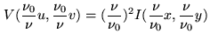 |
(2.42) |
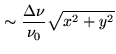
Averaging over the bandwidth
 , there is a radial smearing
equal to
, there is a radial smearing
equal to
 |
(2.43) |
and hence the constraint
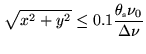 |
(2.44) |
if we want that smearing to be less than 10% of the synthesized beam.
- Time Averaging
Assume for simplicity that the interferometer observes the Celestial Pole.
The baselines cover a sector of
angular width
 , where
  is the Earth rotation
speed, and
is the Earth rotation
speed, and  the integration time. The smearing is
circumferential and of magnitude
the integration time. The smearing is
circumferential and of magnitude
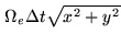 , hence the constraint
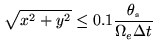 |
(2.45) |
For other declinations, the smearing is no longer rotational, but of similar
magnitude.
To better fix the importance of such approximations, the relevant
values for the Plateau de Bure interferometer are given in Table 2.1.
Table 2.1:
Field of view limitations as function of angular resolution
and observing frequency for the Plateau de Bure interferometer.
| Config. |
Resolution |
Frequency |
2-D |
0.5 GHz |
1 Min Time |
Primary |
| |
|
(GHz) |
Field |
Bandwidth |
Averaging |
Beam |
| Compact |
5 |
80 GHz |
5 |
80 |
2 |
60 |
| Standard |
2 |
80 GHz |
3.5 |
30 |
45 |
60 |
| Standard |
2 |
220 GHz |
3.5 |
1.5 |
45 |
24 |
| High |
0.5 |
230 GHz |
1.7 |
22 |
12 |
24 |
|
Note that these fields of view correspond to a maximum phase error of
6 only, or to a (one dimensional) distortion of a tenth of the
synthesized beam, and thus are not strict limits. In particular,
atmospheric errors often results in larger errors (which are
independent of the field of view, however).
Next: 2.6 Array Geometry &
Up: 2. Millimetre Interferometers
Previous: 2.4 Fringe Stopping and
Contents
Anne Dutrey