3.5 The Feasibility of mm-VLBI: Signal-to-Noise Ratio and Detections

The operation and sensitivity, and the present situation and future wishes of mm-VLBI are easily explained from a discussion of the relation expressing the signal-to-noise ratio of an observation with a two-telescope VLBI interferometer. An unresolved source with a size comparable or smaller than the synthesized beamwidth ($\Theta$), measured with both telescopes (1,2), is considered to be detected if the signal-to-noise ratio (SNR) of the observation is $\sim$7 or higher, i.e. 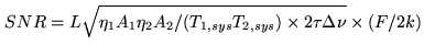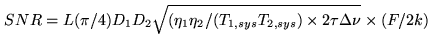7 $\leq$ SNR. The relation of the SNR is ([Rogers et al. 1984])

$$SNR = L \sqrt{\eta_1 A_1 \eta_2 A _2 /(T_{1,sys}T_{2,sys}) \times 2 \tau \Delta \nu} \times (F/2k)$$ (3.4)

$$SNR = L( \pi /4)D_1 D_ 2 \sqrt{(\eta _1 \eta_2 /(T_{1,sys}T_{2,sys}) \times 2 \tau \Delta \nu} \times(F/2k)$$ (3.5)

with A the geometrical area = $\pi$(D/2)$^{2}$ and $\cal D$ the diameter of the telescope (Tables 3.2 &  3.3); $\eta$ the aperture efficiency (Table 3.2); $\eta$A the effective collecting area; T$_{sys}$ the system temperature (Table 3.2); $\Delta$$\nu$ the bandwidth (112MHz for MkIII); $\tau$ the integration time; F the correlated flux density; k the Boltzmann constant; and L the correlator efficiency ($\approx$ 2/$\pi$ for a 2-level quantization). cm From this relation we note that: cm $\bullet$ the incorporation of a large-diameter high-precision telescope significantly improves the performance of a mm-VLBI array. If an array of two telescopes of diameter ${\cal D}_{1} ={\cal D}_{2}$ = 15m and efficiency $\eta_{1} = \eta_{2} = 0.3$ performs at the signal-to-noise ratio SNR(2$\times$15m), the replacement of one telescope by, for instance, the IRAM 30-m telescope with ${\cal D}_{2} = 2$ ${\cal D}_{1}$ = 30m and $\eta_{2} = 2 \eta _{1} = 0.6$ improves the signal-to-noise ratio by SNR(15m & 30m) = 2$\times$SNR(2$\times$15m): the array has a 2 times higher sensitivity. It is evident that the future incorporation of the PdB interferometer, the LMT, and ALMA (Table 3.2) will greatly improve the sensitivity of mm-VLBI. cm $\bullet$ for observations at mm-wavelengths the location of a telescope at 2000-3000m altitude generally reduces T$_{sys}$ because of the lower amount of atmospheric water vapour, i.e. T$_{sys}$(high site) $\approx$ (1/3)$\times$T$_{sys}$(low site) $\approx$ (1/3)$\times$(300-500)K $\approx$ 150K. The lower value of T$_{sys}$ increases the SNR by a factor of 2, or more. Such a decrease of the line-of-sight T$_{sys}$ is especially important for intercontinental/transatlantic baselines where the sources are usually observed at low local elevations (Figure 3.3). Table 3.2 shows that several telescopes of the CMVA array unfortunately are located at low altitudes. Again, the incorporation of PdB Interferometer (2500m), the LMT (4600m), and ALMA (5000m) will greatly improve the sensitivity of mm-VLBI. cm $\bullet$ for continuum observations, the foreseen increase in bandwidth of presently $\Delta$$\nu$ = 112MHz by a factor of two, or more (MkIV), will increase the sensitivity of mm-VLBI by a factor of 1.5, or more. cm $\bullet$ the integration time $\tau$ is usually limited by the stability of the Hydrogen-maser to values $\tau$(100GHz) $\approx$ 1000s and $\tau$(230GHz) $\approx$ 100s (Sect.3.6). Often however, the integration time is shorter, $\tau$(100GHz) $\approx$100-200s and $\tau$(230GHz) $\approx$10-20s, because of phase disturbances introduced by atmospheric water vapour fluctuations. Segmented correlations and atmospheric phase corrections increase the sensitivity of mm-VLBI. cm $\bullet$ the SNR is proportional to the correlated (unresolved) flux density (F) of the source. At mm-wavelengths it is found that the correlated flux density is often significantly smaller than the total flux density (S) measured with a single dish telescope. It is found, globally, that F $\approx$ (1/3-1/5)$\times$S. As example, for 3C273 it is observed that S(86GHz) $\approx$ 20Jy while F(86GHz) $\approx$ 4Jy, and S(230GHz) $\approx$ 10Jy while F(230GHz) $\approx$ 2Jy. The presently available CMVA array has sufficient sensitivity to detect sources of total flux density S $\leq$ 2-3 Jy. cm To illustrate the present situation and possibilities of mm-VLBI, Table 3.6 summarizes the SNR of detections at 86GHz measured on the baseline Pico Veleta (Spain) - Haystack (USA) ([Krichbaum et al. 1994]; [Beasley et al. 1995]).

Table: SNR for 86GHz (3.5mm) Observations: Pico Veleta - Haystack ($\sim$6000km)

Source	S(86GHz) [Jy]	SNR
	(single dish)	(VLBI)
3C273	25	182-203
3C279	20	163
3C345	5.5	6-13
NRAO530	6.5	21-81
1749+096	3.0	21-43
1823+568	2.8	35-43
2145+067	4.5	5-19
3C454.3	10	78-66

Results obtained at 215GHz (1.3mm) on the $\sim$1000km baseline Pico Veleta-PdB are given in Table 3.7 ([Krichbaum et al. 1998]).

Table: SNR for 215GHz (1.3mm) Observations: Pico Veleta - Bure ($\sim$1000km)

Source	z	S(215GHz) [Jy]	SNR	F(215GHz) [Jy]
		(single dish)	(VLBI)	(VLBI)
4C39.25	0.69	3.5$\pm$0.7	$<$ 4	$<$ 0.5
3C273	0.16	9.2$\pm$0.6	7	0.4-0.7
3C279	0.54	11.0$\pm$1.0	35	3-3.8
1334-127	0.54	3.1$\pm$0.7	12	0.5-1.1
3C345	0.59	3.0$\pm$0.4	6	$\leq$ 0.4
NRAO530		6.2$\pm$0.5	11	0.5-0.8
SgrA$^{*}$		4.1$\pm$0.5	6	0.5-0.9