 |
 |
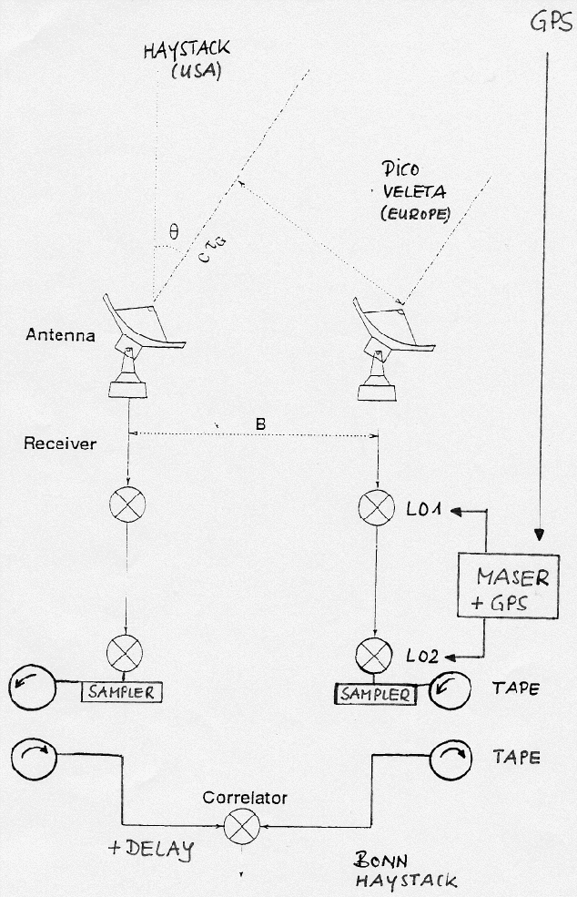
A 2-telescope disconnected mm-VLBI array and the (far away) correlator station are shown in Figure 3.4. mm-VLBI observations are made with telescopes separated by several hundreds or thousands of kilometers not sharing a common time/frequency reference as used in connected interferometry. At each VLBI-telescope therefore the receivers, frequency down-up converters, tape recorders, phase-calibration systems etc. are locked to a Hydrogen-maser which has a typical short-term stability of
In VLBI observations, the telescopes are disconnected and
real-time correlation of the signals from the individual
telescopes is not possible. At each telescope, the signals are
recorded on tape synchronous with the time signal provided by the
Hydrogen-maser. In MkIII mode observations, the data are
available as 28 channels of 4MHz bandwidth each; the bandwidth
of the recording is ![]()
![]() = 28
= 28![]() 4MHz = 112MHz.
The 28 tracks are recorded simultaneously on magnetic tape. The
required bitrate of the recording is
4MHz = 112MHz.
The 28 tracks are recorded simultaneously on magnetic tape. The
required bitrate of the recording is
For ![]()
![]() = 112MHz and a sampling efficiency n
= 112MHz and a sampling efficiency n![]()
![]() 1-1.6, the bitrate recorded on tape is
1-1.6, the bitrate recorded on tape is
![]() 224Megabites/s. mm-VLBI is being upgraded to 256MHz
bandwidth, and more (MkIV).
224Megabites/s. mm-VLBI is being upgraded to 256MHz
bandwidth, and more (MkIV).
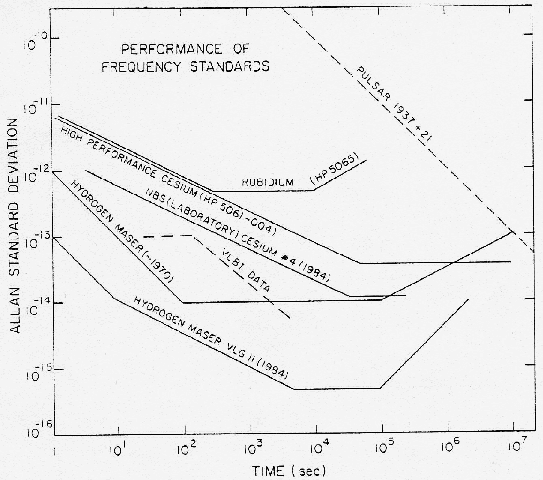
The short-term frequency stability (up to a few 1000s, see
Figure 3.5) of a Hydrogen-maser is ![]() 10
10![]() .
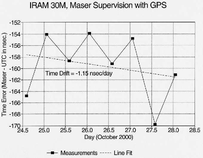
There are long-term drifts which can be checked against GPS
signals (see Figure 3.6) and adjusted so that they are
below, say, ten nano-seconds per day. The maximum possible
integration time (
.
There are long-term drifts which can be checked against GPS
signals (see Figure 3.6) and adjusted so that they are
below, say, ten nano-seconds per day. The maximum possible
integration time (![]() ) of an observation is set by the
requirement that the relative frequency drift
) of an observation is set by the
requirement that the relative frequency drift ![]()
![]() must
not exceed, say,
must
not exceed, say, ![]()
![]()
![]() 0.2 radians. The
integration time then is ([Kellerman & Thompson 1985])
0.2 radians. The
integration time then is ([Kellerman & Thompson 1985])
This relation gives ![]() (86GHz)
(86GHz) ![]() 350s
350s ![]() 5minutes and
5minutes and ![]() (230GHz)
(230GHz) ![]() 150s
150s ![]() 2minutes.
2minutes.
Because of phase variations introduced by atmospheric water vapour
fluctuations, the correlation time ![]() derived above can be
significantly shorter,
derived above can be
significantly shorter, ![]()
![]() 10-30s, especially
when observing at high frequencies. Because of the scarcity of
strong mm-wavelength VLBI sources at sufficiently close distances
in the sky, phase referencing as used in connected mm-wavelength
interferometry (for instance used on PdB) has not yet generally
been applied in mm-VLBI. Efforts are however undertaken to apply
phase corrections from local line-of-sight water vapour
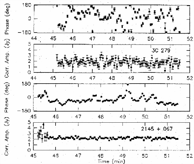
measurements (sky emission measurements). As an example, the phase
stability of a 86GHz and 215GHz measurement between Pico
Veleta and Plateau de Bure is shown in Fig.3.7. A typical
atmosphere-induced phase variation and phase correction applied
to 86GHz VLBI measurements made at Pico Veleta is shown in
Figure 3.8.
10-30s, especially
when observing at high frequencies. Because of the scarcity of
strong mm-wavelength VLBI sources at sufficiently close distances
in the sky, phase referencing as used in connected mm-wavelength
interferometry (for instance used on PdB) has not yet generally
been applied in mm-VLBI. Efforts are however undertaken to apply
phase corrections from local line-of-sight water vapour
measurements (sky emission measurements). As an example, the phase
stability of a 86GHz and 215GHz measurement between Pico
Veleta and Plateau de Bure is shown in Fig.3.7. A typical
atmosphere-induced phase variation and phase correction applied
to 86GHz VLBI measurements made at Pico Veleta is shown in
Figure 3.8.
The recorded mm-wavelength VLBI data are correlated at Haystack (USA) or at Bonn (Germany). The end-product of the correlation are calibrated visibility values (uv-tables) which can be used in the same way as data, for instance, obtained with the PdB interferometer.