3.7 The observable sources with mm-VLBI

3.7.1 Which Kind of sources can we observe

Mm-VLBI sees non-thermal sources emitting, for instance, maser or synchrotron radiation at a high brightness temperature (T$_{\rm B}$). The associated astronomical sources are, for instance, masers (SiO) and AGNs and QSOs with jets. mm-VLBI is insensitive to the cold component of the Universe like molecular clouds and other thermal sources. The cold component is observed with interferometers like the Plateau de Bure instrument. cm The correlated flux density F of a source with brightness temperature T$_{\rm B}$, subtending the solid angle $\Omega$ in the sky, is

$$F = (2k/ \lambda^2) T_B \Omega$$ (3.8)

The correlated flux density $\Delta$F observable within the bandwidth $\Delta$$\nu$ and integration time $\tau$ is

$$\Delta F = (2k/A_{eff}) T_{sys,eff}/ \sqrt{2 \tau \Delta \nu}$$ (3.9)

with A $_{\rm eff}$ = $\sqrt{{\eta}_{1}A_{1}{\eta}_{2}A_{2}}$ the effective surface area of telescope 1$\&$2 and T $_{\rm sys,eff}$ = $\sqrt{T_{1,sys}T_{2,sys}}$ the effective system temperature. To arrive at a numerical value of T$_{\rm B}$ let us assume that we want to detect the source with an accuracy of $\Delta$F $\approx$ $\epsilon$F, where 0 $<$ $\epsilon$ $<$ 1. We assume furthermore that the source is unresolved and small and has a size comparable to the VLBI array resolution, hence $\Omega$ $\approx$ ( $\lambda/\cal B$)$^{2}$. Using these relations we obtain

$$T_B \approx T_{sys,eff} {\cal B}^2 / (\epsilon A \sqrt{2 \tau \Delta \nu})$$ (3.10)

A mm-VLBI array of two telescopes of 15-m diameter, observing at a system temperature T $_{\rm sys,eff}$ = 200K, a bandwidth of $\Delta$$\nu$ = 112MHz, and an integration time limited by the system and atmospheric phase stability to $\tau$ $\approx$ 100s, can only detect sources which have brightness temperatures of T$_{\rm B}$ $\approx$ 10$^{9}$ - 10$^{12}$K.

3.7.2 The field of view

Evidently, a mm-VLBI array of 8000-10000km baseline has only a limited field of view ($\theta$ $_{\rm fov}$). Since a disconnected mm-VLBI array does not directly track phase, an estimate of the field of view is obtained by noting that the delay $\tau$ between two antennas (see Figure 3.4) separated by the baseline B and observing in the direction $\theta$

$$\tau = ({\cal B}/c) \cos{\theta}$$ (3.11)

and that the delay difference $\Delta$$\tau$ for a small angular displacement $\Delta$$\theta$ from the main direction of observation is

$$\Delta \tau = - ({\cal B}/c) \sin{\theta}) \Delta \theta$$ (3.12)

with c the velocity of light. Since delay corrections are only made in the correlator, the field of view is restricted to directions in which delay smearing ($\Delta$$\tau$) does not exceed, approximately, $\Delta$$\tau$ $\leq$ 1/(2$\Delta$$\nu$). Using this criterion, the field of view is

$$\theta_{fov} \approx \lambda/{\cal B} (\nu/ \Delta \nu)$$ (3.13)

For $\nu$ = 86GHz, $\Delta$$\nu$ = 112MHz (MkIII), and $\cal B =$ 10000km we obtain $\theta$ $_{\rm fov}$ $\approx$ 0.05-0.02$''$ $\equiv$ 50-20 mas.

$\parbox{150mm}{ \caption{Figure 3.8: mm... ...n into account (by courtesy of M. Bremer, IRAM, A. Roy and D. Graham, MPIfR).}}$

3.7.3 An example: mm-VLBI Observations of QSO 3C273

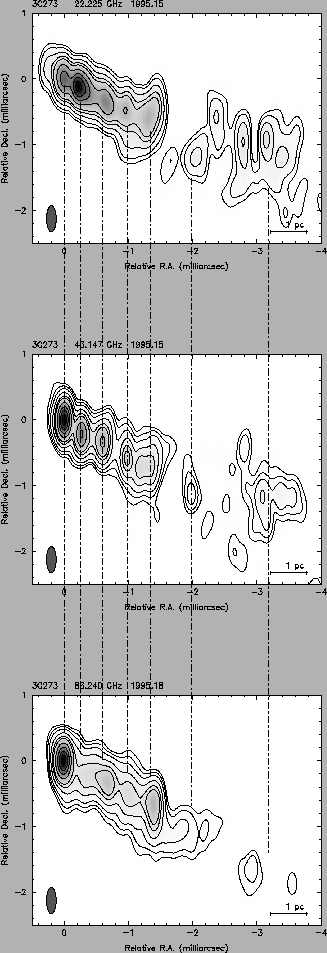
Fig.3.9 shows observations of the Quasar 3C273 at 22GHz (top), 43GHz (center), and 86GHz (bottom), performed nearly at the same epochs of 1995.15 (22 and 43GHz) and 1995.18 (86GHz). Contour levels in all maps are (-0.5,) 0.5, 1, 2, 5, 10, 15, 30, 50, 70, and 90% of the peak flux density of 3.0Jy/beam (top), 5.4Jy/ (center), and 4.7Jy/beam (bottom). All maps are restored with the same beam of size of $0.4  {\rm x}  0.15$mas, oriented at $\rm {pa}= 0^{\rm o}$. The maps are arbitrarily centered on the eastern component (the core); the dashed lines guide the eye and help to identify corresponding jet components in the three maps.

$\parbox{50mm}{ \caption{Figure 3.9: VLB... ...d from observations with the CMVA array (by courtesy of T. Krichbaum, MPIfR).}}$