6.1 Introduction

As we already learned in the lecture on radio interferometry by S.Guilloteau (Chapter 2), the interferometer measures the complex cross-correlation function of the voltage at the outputs of a pair of antennas $(i,j)$. This quantity, $R_{\rm ij}({\tau})$ is defined as

$$R_{\rm ij}({\tau}) = \langle v_i(t) v_j(t+\tau) \rangle$$ (6.1)

(the brackets indicate the time average, see AppendixA). The cross-correlation function is related to the visibility function $V = \vert V\vert\exp{(i\ensuremath{\varphi_\mathrm{\scriptscriptstyle SKY}})}$ by

$$R_{\rm ij} = A_0 \vert V\vert \Delta \ensuremath{\nu_\mathrm{\scr... ...criptscriptstyle \rm G}}-\ensuremath{\varphi_\mathrm{\scriptscriptstyle SKY}})}$$ (6.2)

where $A_0$ is the collecting area of the antenna. Eq.6.2 only holds for a quasi-monochromatic signal, $\Delta\ensuremath{\nu_\mathrm{\scriptscriptstyle IF}} \ll \ensuremath{\nu_\mathrm{\scriptscriptstyle IF}}$ (i.e. the bandpass may be represented by a $\delta$-function). The signal phase varies with time due to source structure and atmospheric perturbations (expressed by $\ensuremath{\varphi_\mathrm{\scriptscriptstyle SKY}}$), and due to the geometric delay $\ensuremath{\tau_\mathrm{\scriptscriptstyle \rm G}}$. The timescale that is needed to fully sample a spectral line, given by the sampling theorem (see below), is much shorter. Here are examples of the different timescales:

1. timescale for phase variation by $1^\circ$ due to source structure (for a point source at 100GHz with $\Delta\alpha = 10''$ offset from phase reference center, east-west baseline of 180m during transit): 10min
2. timescale for phase variation due to atmospheric perturbations: (depending on atmospheric conditions and baseline length): 1sec - several hours
3. sampling time step for a 80 MHz bandwidth: 6.25ns
4. maximum time lag needed for a 40 kHz resolution: 25 $\mathbf{\mu}$s

The sampling time step in the above example is that short that the signal will be dominated by noise. Any deterministic contribution will show in the correlation products. We have to assume that the noise is due to a stationary random process (within a time interval given by the maximum time lag).


In the following, I will discuss digital techniques to evaluate $R_{\rm ij}({\tau})$. Analog methods of signal processing are highly impractical in radio interferometry, for mainly two reasons:

1. In time domain, high precision is needed.
2. The signal needs to be identically copied, in order to cross-correlate the output of one antenna with the outputs from all other antennas. This can be more easily done with digital techniques, than with analog ones.

The first signal processing steps are analog, beginning with the mixing in the heterodyne receivers. For reasons that will become clear later (see R.Lucas, Chapter 7), only the case of single-sideband reception is considered. The sidebands may be separated by a periodic phase shift of $\pi/2$ applied to the local oscillator. The signals are demodulated in two different ways by the correlator. At the entry of the correlator, filters are inserted, that are used to select the intermediate frequency bandpass. The following signal processing steps are digitally implemented, and are performed within the correlator:

1. Sampling the signal: in order to digitize the signal, it needs to be sampled. Bandwidth-limited signals (i.e. containing frequencies between zero and $\Delta \nu$) may be sampled without loss of information if the samples are taken at time intervals $\Delta t \le 1/(2\Delta\nu)$.
2. In order to numerically compute the cross correlation function, the signals have to be discretized. The data are affected by such a quantization, but may be corrected for it. However, the loss of information cannot be recovered and degrades the correlator sensitivity.
3. Delay compensation: the geometric delays are eliminated for signals received from the direction of the pointing center. Remaining delays are due to source structure.
4. Until now, everything is done in the time domain. However, for spectroscopic applications, the desired output is the cross power spectral density, and not the cross correlation function. These quantities are Fourier-transform pairs (Wiener-Khintchine theorem) ^6.1. The transformation can be efficiently done by a processor performing a Fast Fourier Transform.

The plan of this lecture is as follows: after the basic theory, I will talk about the correlator in practice. Both the intrinsic limitations and system-dependent performance will be discussed. For further reading, the book of [Thompson et al. 1986] (chapters 6 - 8), and the introduction by [D'Addario 1989] are recommended. Finally, as an example, the current correlator system on Plateau de Bure will be presented.

Figure 6.1: Architecture of a complex continuum cross correlator.

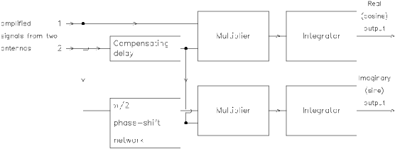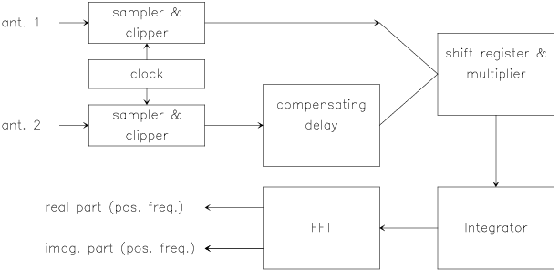
Figure 6.2: Architecture of a complex spectroscopic cross correlator.