Next: 6.3 The Correlator in
Up: 6. Cross Correlators
Previous: 6.1 Introduction
Contents
The ``heart'' of a correlator consists of the sampler and the cross-correlator.
Eq.6.2 represents an over-simplified case, because the bandwidth
of the signals is neglected. The correlator output is rather modified by the
Fourier transform of the bandpass function. For the sake of simplicity,
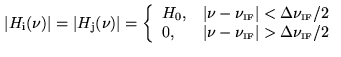
let us assume an idealized rectangular passband of width
 for both antennas, centered at the intermediate frequency
 , i.e.
(this assumption will be relaxed later).
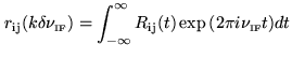
The correlator response to this bandpass is the Fourier transform of the
cross power spectrum
 , which is
shown in Fig.6.3:
, which is
shown in Fig.6.3:
 |
(6.3) |
The correlator output consists of an oscillating part, and a
 envelope (a sinc function). If the delay
  becomes too large, the
sensitivity will be significantly decreased due to the sinc function (see
Fig.6.3). Strictly speaking, this is the response to the real
part of the bandpass, which is symmetric with respect to negative frequencies.
The imaginary part of the bandpass is antisymmetric with respect to
negative frequencies, thus the correlator response is different. The separation
of real and imaginary parts in continuum and spectroscopic correlators will be
discussed below.
becomes too large, the
sensitivity will be significantly decreased due to the sinc function (see
Fig.6.3). Strictly speaking, this is the response to the real
part of the bandpass, which is symmetric with respect to negative frequencies.
The imaginary part of the bandpass is antisymmetric with respect to
negative frequencies, thus the correlator response is different. The separation
of real and imaginary parts in continuum and spectroscopic correlators will be
discussed below.
This example shows that accurate delay tracking (fringe stopping)
is needed, if the bandwidth is not anymore negligible with respect
to the intermediate frequency. In other words, the compensating
delay
 needs to keep the delay tracking error
 at a minimum. The
offset
at a minimum. The
offset  introduced in correlator channel
  needs to
be applied with respect to a fixed delay. In the following, the
correlator response to a rectangular bandpass will be expressed by
the more general instrumental gain function
needs to
be applied with respect to a fixed delay. In the following, the
correlator response to a rectangular bandpass will be expressed by
the more general instrumental gain function
 ,
defined by
,
defined by
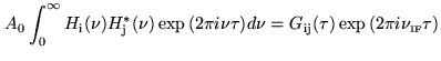 |
(6.4) |
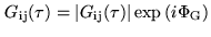 is a complex
quantity, including phase shifts due to the analog part of the receiving
system (amplificators, filters)6.2. After fringe stopping, the single-sideband response of
correlator channel becomes (for details, see R.Lucas, Chapter 7)
is a complex
quantity, including phase shifts due to the analog part of the receiving
system (amplificators, filters)6.2. After fringe stopping, the single-sideband response of
correlator channel becomes (for details, see R.Lucas, Chapter 7)
where the plus sign refers to upper sideband reception, and the minus sign
refers to lower sideband reception. From Eq.6.6, we immediately
see that the residual delay error (due to a non-perfect delay tracking)
enters as a constant phase slope across the bandpass (with opposed signs
in the upper and lower sidebands). The effect of such a phase slope on
sensitivity will be discussed later. In order to determine the phase
of the signal, the imaginary part of
 has to be
simultaneously measured. In a continuum correlator (Fig.6.1),
a
has to be
simultaneously measured. In a continuum correlator (Fig.6.1),
a  phase shift applied to the analog signal yields the imaginary part.
The signals are then separately processed by a cosine and a sine correlator
6.3.
In other words: the pattern shown in Fig.6.3 is measured
in the close vicinity of two points, namely at the origin, and at
a quarter wave later, i.e. at
phase shift applied to the analog signal yields the imaginary part.
The signals are then separately processed by a cosine and a sine correlator
6.3.
In other words: the pattern shown in Fig.6.3 is measured
in the close vicinity of two points, namely at the origin, and at
a quarter wave later, i.e. at
 . Note,
however, that due to the sinc-envelope, the decreasing response function
cannot be neglected if the bandwidth is comparable to the intermediate
frequency.
. Note,
however, that due to the sinc-envelope, the decreasing response function
cannot be neglected if the bandwidth is comparable to the intermediate
frequency.
In a spectroscopic correlator (Fig.6.2), the
imaginary part can be entirely deduced from the digitized
signal: if
 is the number of complex spectral channels,
 time lags are used, covering delays from
 to
to
 .
The correlator output is a real signal with even and odd components (with
respect to time lags of opposed signs). The
.
The correlator output is a real signal with even and odd components (with
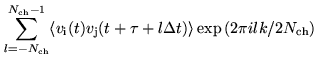
respect to time lags of opposed signs). The  complex channels of the
Fourier transform at positive frequencies yields the cross-power spectrum:
complex channels of the
Fourier transform at positive frequencies yields the cross-power spectrum:
(for channel of a total of
complex channels,
spaced by
 ). The last expression represents the
discrete Fourier transform. According to the symmetry properties
of Fourier transforms, the even component of the correlator output
becomes the real part of the complex spectrum, and the odd
component becomes the imaginary part. The Fourier transform is
efficiently evaluated using the Fast-Fourier algorithm. In
practice, it is rather the digital measurement of the
cross-correlation function that is non-trivial. It will be
discussed in detail in Section 6.3.3.
). The last expression represents the
discrete Fourier transform. According to the symmetry properties
of Fourier transforms, the even component of the correlator output
becomes the real part of the complex spectrum, and the odd
component becomes the imaginary part. The Fourier transform is
efficiently evaluated using the Fast-Fourier algorithm. In
practice, it is rather the digital measurement of the
cross-correlation function that is non-trivial. It will be
discussed in detail in Section 6.3.3.
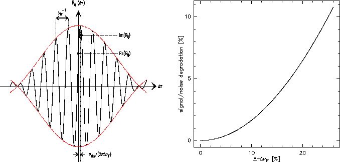
Figure:
Left:
Correlator output (single-sideband reception) for a rectangular
passband with
 . Due to the signal
phase
. Due to the signal
phase
 , the oscillations move through the sinc envelope
by
, the oscillations move through the sinc envelope
by
 . The shift may also be due to the
phase of the complex gain (in this case, the shift would be in
opposed sense for USB and LSB reception). Right: Sensitivity
degradation due to a delay error
. The shift may also be due to the
phase of the complex gain (in this case, the shift would be in
opposed sense for USB and LSB reception). Right: Sensitivity
degradation due to a delay error
 (with respect to
the inverse IF bandwidth). The effect is due to the fall-off of
the sinc envelope.
(with respect to
the inverse IF bandwidth). The effect is due to the fall-off of
the sinc envelope.
 |
The ensemble of cross-power spectra
 , after
tracking the source for some time, becomes (after calibration and several
imaging processes) a channel map.
, after
tracking the source for some time, becomes (after calibration and several
imaging processes) a channel map.
Next: 6.3 The Correlator in
Up: 6. Cross Correlators
Previous: 6.1 Introduction
Contents
Anne Dutrey