next up previous contents
Next: 7.2 Delay lines requirements Up: 7. LO System and Previous: 7. LO System and   Contents

Subsections

7.1 An Heterodyne Interferometer

7.1.1 The simple interferometer

This is composed of 2 antennas, a multiplier, an integrator (Fig. 7.1); we directly multiply the signals, and average in time. $ \ensuremath{\tau_\mathrm{\scriptscriptstyle G}} = 2\pi \ensuremath{\text{\boldmath $b$\unboldmath }}. \ensuremath{\text{\boldmath $s$\unboldmath }}/c$ is the geometrical delay.

Figure 7.1: A simple, two-antenna interferometer
\resizebox{8cm}{!}{\includegraphics{rl1fig1.eps}}

Provided the geometrical delay is compensated in the hardware, after filtering out the high frequency terms, the output of the correlator is the real part of the visibility:

$\displaystyle r(t) = A \cos{\ensuremath{\varphi_\mathrm{\scriptscriptstyle }}(t)}$ (7.1)

A complex correlator using a quadrature network can be used to measure the imaginary part; or (equivalently) one uses a spectral correlator.

7.1.2 The heterodyne interferometer

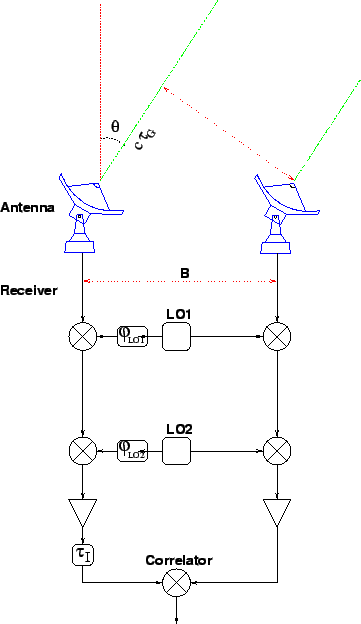
We now consider a more realistic two antenna system (Fig. 7.2), which includes two frequency conversions: e.g. one in the SIS mixer, and one to move the IF band to baseband for numerical sampling and digital correlation. This again is a simplification, but includes all the important effects. The PdB system has in fact 4 frequency conversions (see below).

Figure 7.2: A heterodyne, two-antenna interferometer, with two frequency conversions
\resizebox{8cm}{!}{\includegraphics{rl1fig2b.eps}}

Let us first consider the effect on phase of a simple frequency conversion.

7.1.3 Frequency conversion

The input signal to the mixer is $ U(t) = E \cos{(\omega t +
\phi)}$, and the first LO signal (LO1) is $ \ensuremath{U_\mathrm{\scriptscriptstyle LO1}}(t) = \ensuremath{E_\mathrm{\scr...
...iptscriptstyle LO1}} t +
\ensuremath{\varphi_\mathrm{\scriptscriptstyle LO1}})}$. Mixer output is proportional to $ [U(t)+\ensuremath{U_\mathrm{\scriptscriptstyle LO1}}(t)]^2$ and we select by a filter a band $ \Delta \omega$ centered on $ \omega_\mathrm{\scriptscriptstyle IF}$. We note: $ \ensuremath{\omega_\mathrm{\scriptscriptstyle U}} = \ensuremath{\omega_\mathrm{\scriptscriptstyle LO1}} + \ensuremath{\omega_\mathrm{\scriptscriptstyle IF}}$, and $ \ensuremath{\omega_\mathrm{\scriptscriptstyle L}} = \ensuremath{\omega_\mathrm{\scriptscriptstyle LO1}} - \ensuremath{\omega_\mathrm{\scriptscriptstyle IF}}$ the angular frequencies in the upper sideband and in the lower sideband, respectively.
The IF output is
$\displaystyle \ensuremath{U_\mathrm{\scriptscriptstyle IF}}(t)$ $\displaystyle \propto$ $\displaystyle \ensuremath{E_\mathrm{\scriptscriptstyle U}}\cos{[(\ensuremath{\o...
...m{\scriptscriptstyle L}}+\ensuremath{\varphi_\mathrm{\scriptscriptstyle LO1}}]}$  
$\displaystyle \ensuremath{U_\mathrm{\scriptscriptstyle IF}}(t)$ $\displaystyle \propto$ $\displaystyle \ensuremath{E_\mathrm{\scriptscriptstyle U}}\cos{(\ensuremath{\om...
...m{\scriptscriptstyle L}}+\ensuremath{\varphi_\mathrm{\scriptscriptstyle LO1}})}$ (7.2)

After the frequency conversion the phase is the difference of the signal phase and the LO phase, with a sign reversal if the conversion is lower sideband:
  USB LSB
frequency: $ \ensuremath{\omega_\mathrm{\scriptscriptstyle IF}}=\ensuremath{\omega_\mathrm{\scriptscriptstyle U}}-\ensuremath{\omega_\mathrm{\scriptscriptstyle LO1}}$ $ \ensuremath{\omega_\mathrm{\scriptscriptstyle IF}}=-\ensuremath{\omega_\mathrm{\scriptscriptstyle L}}+\ensuremath{\omega_\mathrm{\scriptscriptstyle LO1}}$
phase: $ \ensuremath{\varphi_\mathrm{\scriptscriptstyle IF}} = \ensuremath{\varphi_\mathrm{\scriptscriptstyle U}}-\ensuremath{\varphi_\mathrm{\scriptscriptstyle LO1}}$ $ \ensuremath{\varphi_\mathrm{\scriptscriptstyle IF}}
=-\ensuremath{\varphi_\mathrm{\scriptscriptstyle L}}+\ensuremath{\varphi_\mathrm{\scriptscriptstyle LO1}} $

7.1.4 Signal phase

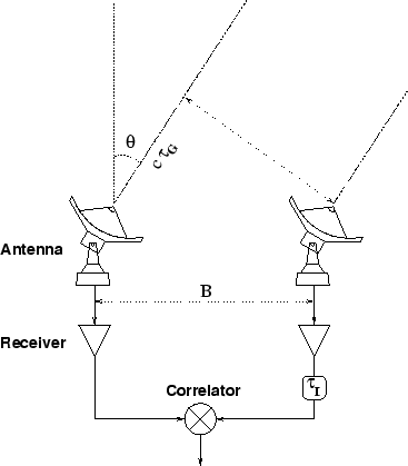
One antenna is affected by the geometrical delay $ \tau_\mathrm{\scriptscriptstyle G}$, and by the phase ( $ \varphi_\mathrm{\scriptscriptstyle U}$ in the upper sideband, $ \varphi_\mathrm{\scriptscriptstyle L}$ in the lower sideband), which is the quantity to be measured. We apply a compensating delay $ \tau_\mathrm{\scriptscriptstyle I}$ in the second IF (IF2), as well as a phase $ \varphi_\mathrm{\scriptscriptstyle LO1}$ to the first LO and a phase $ \varphi_\mathrm{\scriptscriptstyle LO2}$ on the second LO (LO2). We note $ \Delta\tau = \ensuremath{\tau_\mathrm{\scriptscriptstyle I}}+\ensuremath{\tau_\mathrm{\scriptscriptstyle G}}$ the delay tracking error. In a 2-antenna system, we may assume that the signal path through the first antenna suffers no delay of phase offset terms. Obviously the compensating delay $ \tau_\mathrm{\scriptscriptstyle I}$ in the second antenna may need to be negative, if the second antenna is closer to the source: in that case one will apply the positive delay $ -\ensuremath{\tau_\mathrm{\scriptscriptstyle I}}$ on the first antenna. In a $ N$ antenna system, one will apply phase and delay commands to all the antennas; a common delay will be applied to all the antennas since no negative delay can be built with current technology.

Let us first consider the upper sideband of the first LO (second LO conversion is assumed upper sideband for simplicity):

  USB LSB
HF Frequency (RF) $ \omega_\mathrm{\scriptscriptstyle USB}$ $ \omega_\mathrm{\scriptscriptstyle L}$
HF Phase $ \ensuremath{\varphi_\mathrm{\scriptscriptstyle U}}+\ensuremath{\omega_\mathrm{\scriptscriptstyle U}}\ensuremath{\tau_\mathrm{\scriptscriptstyle G}}$ $ \ensuremath{\varphi_\mathrm{\scriptscriptstyle L}}+\ensuremath{\omega_\mathrm{\scriptscriptstyle L}}\ensuremath{\tau_\mathrm{\scriptscriptstyle G}}$
LO1 Frequency $ \omega_\mathrm{\scriptscriptstyle LO1}$ $ \omega_\mathrm{\scriptscriptstyle LO1}$
LO1 Phase $ \varphi_\mathrm{\scriptscriptstyle LO1}$ $ \varphi_\mathrm{\scriptscriptstyle LO1}$
IF1 Frequency $ \ensuremath{\omega_\mathrm{\scriptscriptstyle IF1}}=\ensuremath{\omega_\mathrm{\scriptscriptstyle U}}-\ensuremath{\omega_\mathrm{\scriptscriptstyle LO1}}$ $ \ensuremath{\omega_\mathrm{\scriptscriptstyle IF1}}=\ensuremath{\omega_\mathrm{\scriptscriptstyle LO1}}-\ensuremath{\omega_\mathrm{\scriptscriptstyle L}}$
IF1 Phase $ \ensuremath{\varphi_\mathrm{\scriptscriptstyle U}}+\ensuremath{\omega_\mathrm{...
...hrm{\scriptscriptstyle G}}-\ensuremath{\varphi_\mathrm{\scriptscriptstyle LO1}}$ $ -\ensuremath{\varphi_\mathrm{\scriptscriptstyle L}}-\ensuremath{\omega_\mathrm...
...hrm{\scriptscriptstyle G}}+\ensuremath{\varphi_\mathrm{\scriptscriptstyle LO1}}$
LO2 Frequency $ \omega_\mathrm{\scriptscriptstyle LO2}$ $ \omega_\mathrm{\scriptscriptstyle LO2}$
LO2 Phase $ \varphi_\mathrm{\scriptscriptstyle LO2}$ $ \varphi_\mathrm{\scriptscriptstyle LO2}$
IF2 Frequency $ \ensuremath{\omega_\mathrm{\scriptscriptstyle IF2}}=\ensuremath{\omega_\mathrm...
...m{\scriptscriptstyle LO1}}-\ensuremath{\omega_\mathrm{\scriptscriptstyle LO2}} $ $ \ensuremath{\omega_\mathrm{\scriptscriptstyle IF2}}=\ensuremath{\omega_\mathrm...
...hrm{\scriptscriptstyle L}}-\ensuremath{\omega_\mathrm{\scriptscriptstyle LO2}} $
IF2 Phase $ \ensuremath{\varphi_\mathrm{\scriptscriptstyle U}}+\ensuremath{\omega_\mathrm{...
...m{\scriptscriptstyle LO1}}-\ensuremath{\varphi_\mathrm{\scriptscriptstyle LO2}}$ $ -\ensuremath{\varphi_\mathrm{\scriptscriptstyle L}}-\ensuremath{\omega_\mathrm...
...m{\scriptscriptstyle LO1}}-\ensuremath{\varphi_\mathrm{\scriptscriptstyle LO2}}$
after $ \tau_\mathrm{\scriptscriptstyle I}$ $ \ensuremath{\varphi_\mathrm{\scriptscriptstyle U}}+\ensuremath{\omega_\mathrm{...
...\mathrm{\scriptscriptstyle IF2}}\ensuremath{\tau_\mathrm{\scriptscriptstyle I}}$ $ -\ensuremath{\varphi_\mathrm{\scriptscriptstyle L}}-\ensuremath{\omega_\mathrm...
...mathrm{\scriptscriptstyle IF2}}
\ensuremath{\tau_\mathrm{\scriptscriptstyle I}}$
Final $ \ensuremath{\varphi_\mathrm{\scriptscriptstyle U}}+\ensuremath{\omega_\mathrm{\scriptscriptstyle IF2}}\Delta\tau$ $ -\ensuremath{\varphi_\mathrm{\scriptscriptstyle L}}+\ensuremath{\omega_\mathrm{\scriptscriptstyle IF2}}\Delta\tau$
  $ -(\ensuremath{\varphi_\mathrm{\scriptscriptstyle LO1}}+\ensuremath{\omega_\mathrm{\scriptscriptstyle LO1}}\ensuremath{\tau_\mathrm{\scriptscriptstyle G}})$ $ +(\ensuremath{\varphi_\mathrm{\scriptscriptstyle LO1}}+\ensuremath{\omega_\mathrm{\scriptscriptstyle LO1}}\ensuremath{\tau_\mathrm{\scriptscriptstyle G}})$
  $ -(\ensuremath{\varphi_\mathrm{\scriptscriptstyle LO2}}+\ensuremath{\omega_\mathrm{\scriptscriptstyle LO2}}\ensuremath{\tau_\mathrm{\scriptscriptstyle G}})$ $ -(\ensuremath{\varphi_\mathrm{\scriptscriptstyle LO2}}+\ensuremath{\omega_\mathrm{\scriptscriptstyle LO2}}\ensuremath{\tau_\mathrm{\scriptscriptstyle G}})$

To stop the fringes in both sidebands we need the following conditions:

$\displaystyle \Delta\tau = \ensuremath{\tau_\mathrm{\scriptscriptstyle I}}+\ensuremath{\tau_\mathrm{\scriptscriptstyle G}}$ $\displaystyle =$ 0 (7.3)
$\displaystyle \ensuremath{\varphi_\mathrm{\scriptscriptstyle LO1}}+\ensuremath{...
...\mathrm{\scriptscriptstyle LO1}}\ensuremath{\tau_\mathrm{\scriptscriptstyle G}}$ $\displaystyle =$ 0 (7.4)
$\displaystyle \ensuremath{\varphi_\mathrm{\scriptscriptstyle LO2}}+\ensuremath{...
...\mathrm{\scriptscriptstyle LO2}}\ensuremath{\tau_\mathrm{\scriptscriptstyle G}}$ $\displaystyle =$ 0 (7.5)

One sees that delay tracking in the second IF imposes a phase tracking on the first and second oscillators. The delay error $ \Delta \tau $ appears as a phase term proportional to frequency in the IF2 band $ \omega_\mathrm{\scriptscriptstyle IF2}$.

The condition that e.g. $ \ensuremath{\varphi_\mathrm{\scriptscriptstyle LO1}} = -\ensuremath{\omega_\mathrm{\scriptscriptstyle LO1}}\ensuremath{\tau_\mathrm{\scriptscriptstyle G}}$ means that $ \varphi_\mathrm{\scriptscriptstyle LO1}$ must be commanded to vary at a rate
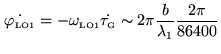
$\displaystyle \dot{\ensuremath{\varphi_\mathrm{\scriptscriptstyle LO1}}} = -\en...
..._\mathrm{\scriptscriptstyle G}}} \sim 2\pi\frac{b}{\lambda_1}\frac{2\pi}{86400}$ (7.6)

which is about 10 turns per second for $ \lambda_1=1$mm and $ b=1$km. The condition is much easier for the second LO. In practice the phase is commanded typically every second, as well as its rate of change during the next second (the real curve is approximated by a piecewise linear curve). Note that a linear drift with time of the phase is strictly equivalent to a small frequency offset.


next up previous contents
Next: 7.2 Delay lines requirements Up: 7. LO System and Previous: 7. LO System and   Contents
Anne Dutrey