The astronomical setup of the interferometer involves a number of steps that are done under the joint responsibility of the array operator and of the astronomer on duty (AoD). The goal of the setup is to maximize the interferometer performance in view of sensitivity and positional precision.
A change of configuration is the responsibility of the operators and of the technical
staff. Since most projects, as mapping, mosaicing and snapshot observations, require more
uv-coverage than a single configuration can provide, the antennas are moved
typically every three weeks or so, to a new configuration. Every additional configuration
increases the mapping sensitivity and the uniformity of the uv-coverage by adding
![]() baselines to the sampling function (these are 10 baselines during the winter
period, 6 baselines during the summer period when the array is operated with only 4
antennas). Configurations are usually selected among six types according to several
criteria: antenna availability, project type, atmospheric seeing, uv-coverage,
pressure in local sidereal time, sun avoidance and other factors.
baselines to the sampling function (these are 10 baselines during the winter
period, 6 baselines during the summer period when the array is operated with only 4
antennas). Configurations are usually selected among six types according to several
criteria: antenna availability, project type, atmospheric seeing, uv-coverage,
pressure in local sidereal time, sun avoidance and other factors.
Six primary configurations are needed to cover the desired range of angular resolution at the two operating frequencies with 5 antennas:
| Configuration | Stations |
| D | W05 W00 E03 N05 N09 |
| C1 | W05 W01 E10 N07 N13 |
| C2 | W12 W09 E10 N05 N15 |
| B1 | W12 E18 E23 N13 N20 |
| B2 | W23 W12 E12 N17 N29 |
| A | W27 W23 E16 E24 N29 |
| Set | Configurations | Purpose |
| D | D | detection / lowest resolution |
| CD | D, C2 or C1 | 3.5 |
| CC | C1, C2 | higher resolution than CD |
| BC | B1, C2 | 2.0 |
| BB | B1, B2, C2 | higher resolution and sensitivity |
| AB | A, B1, B2 | 1.0 |
Special configurations and sets of configurations are used during the annual antenna maintenance period which is usually between May and October. During this period observations at 1mm are for most of the time not feasible, specially in the two extended B configurations. Observations in the A configuration whether at 3mm or 1mm will in general only be scheduled during the winter period. Requested non-standard configurations are considered only in exceptional cases.
Sensitivity is one of the most important concerns. As a rule of thumb, an axial
displacement of the secondary by
![]() results in a 20% loss of
sensitivity. To avoid losses larger than 3%, the position of the secondary needs to be
measured to much better than
results in a 20% loss of
sensitivity. To avoid losses larger than 3%, the position of the secondary needs to be
measured to much better than
![]() on regular time intervals. The positional
precision, however, depends on the source strength, the operating wavelength, the sampling
of secondary positions and, finally, on atmosphere stability. In general, the focus is
measured at 3mm on a strong quasar by displacing the secondary in steps of 1mm (in
steps of 0.45mm if done at 1mm). This is systematically done by the operators at the
beginning of every project and is automatically verified by the system every hour during
project execution.
on regular time intervals. The positional
precision, however, depends on the source strength, the operating wavelength, the sampling
of secondary positions and, finally, on atmosphere stability. In general, the focus is
measured at 3mm on a strong quasar by displacing the secondary in steps of 1mm (in
steps of 0.45mm if done at 1mm). This is systematically done by the operators at the
beginning of every project and is automatically verified by the system every hour during
project execution.
A high pointing accuracy is demanded in view of sensitivity and mapping quality. Antenna
pointing errors affect the global sensitivity of the interferometer and may lead to severe
errors in the image restoration process. As a rule, a pointing precision of
![]() is desirable at the highest frequency. The good
pointing accuracy results from an optimized structural design: a good knowledge of the
gravitational load, a good positional stability of the receivers (a good alignment is
needed for dual-frequency observations), a precise control of the secondary, high
precision bearings and position encoders, a good servo system,
is desirable at the highest frequency. The good
pointing accuracy results from an optimized structural design: a good knowledge of the
gravitational load, a good positional stability of the receivers (a good alignment is
needed for dual-frequency observations), a precise control of the secondary, high
precision bearings and position encoders, a good servo system, ![]() and a good
software control for repeatable antenna pointing errors. The quality of a pointing model
is generally limited by wind and thermal load effects. The absolute pointing accuracy
achievable with the IRAM antennas is in general below the 2-3
and a good
software control for repeatable antenna pointing errors. The quality of a pointing model
is generally limited by wind and thermal load effects. The absolute pointing accuracy
achievable with the IRAM antennas is in general below the 2-3![]() rms at each axis with a
slightly higher uncertainty in elevation. Such a pointing accuracy leads to very small
intensity variations, most of the time with negligible effects on the image
reconstruction. Higher accuracy is obtained by regular relative pointing measurements
every hour.
rms at each axis with a
slightly higher uncertainty in elevation. Such a pointing accuracy leads to very small
intensity variations, most of the time with negligible effects on the image
reconstruction. Higher accuracy is obtained by regular relative pointing measurements
every hour.
Each antenna is characterized by a fixed set of pointing parameters. These are measured only in certain circumstances: when an antenna is going to see first light, when modifications are made which may affect the pointing of an antenna, or more generally in cases of suspected pointing problems. In these cases a precise interferometric pointing session, eventually with a preceding less sensitive full-sky single-dish session, is required to derive the full set of antenna pointing parameters. Such pointing sessions are reduced with a dedicated non-linear fitting program in use at Plateau de Bure.
The pointing model is actually based on 5 parameters only, all others being negligibly
small. These parameters are: IAZ and IEL (the azimuth and elevation encoder zero point
correction), COH (the antenna horizontal collimation), and IVE and IVN (the antenna
East-West and North-South inclination). IAZ, IEL, IVE and IVN are in station dependent,
while COH is in principle an antenna constant. IAZ, IEL and COH are measured in
interferometric mode by pointing on a few low elevation and high elevation sources. In
general, three strong quasars at 3mm are fully sufficient. The remaining two parameters,
IVE and IVN are measured on every project start with an inclinometer by making an antenna
turn through 360![]() .
.
Delay measurements aim at the correction of cable length (electric path) differences between two antennas after compensation of the geometrical path length. An improper knowledge of the difference in cable length is visible as a frequency dependent phase slope in the intermediate frequency bands (IF1 and IF2), and, depending on the amplitude of the slope, may result in a more or less important loss of sensitivity. The delay is measured by a cross-correlation on a strong radio source at the beginning of every project.
The goal is to measure the position of each antenna ![]() relative
to a common reference point (distances
relative
to a common reference point (distances
![]() between antennas
between antennas ![]() and
and ![]() or distances
or distances
![]() with
respect to the theoretical station position) in order to subtract
the phase term
with
respect to the theoretical station position) in order to subtract
the phase term ![]() (see Chapter 2 by
S.Guilloteau) at any hour angle and declination from the observed
phase. The absence of a good baseline solution is equivalent to
having large uncertainties in the baseline separation between
different antennas. As a consequence, the geometrical delay might
improperly be compensated and large time-variable phase errors
might affect the observations.
(see Chapter 2 by
S.Guilloteau) at any hour angle and declination from the observed
phase. The absence of a good baseline solution is equivalent to
having large uncertainties in the baseline separation between
different antennas. As a consequence, the geometrical delay might
improperly be compensated and large time-variable phase errors
might affect the observations.
Though the quality of a baseline solution is easily found out - the calibrator's
visibility phase shouldn't vary with reference to the phase tracking center as function of
hour angle and declination - a good baseline solution is truly indispensable for the
purpose of phase calibration. Phase errors can often be more deleterious on compact
configurations where source visibilities are stronger than on extended configurations. As
a reference, winter conditions allow baselines in the D configuration to be measured at
3mm with a
![]() phase accuracy and with
phase accuracy and with
![]() in the A
configuration. In summer conditions the accuracy is often
in the A
configuration. In summer conditions the accuracy is often ![]() times lower.
times lower.
Though no high accuracy is needed for antenna positioning (offset position from the target
location is routinely within a wavelength), the actual antenna position has to be known
with high precision: within a small fraction of a wavelength (70-300![]() m). The precision
is limited essentially by the atmosphere and by thermal effects.
m). The precision
is limited essentially by the atmosphere and by thermal effects.
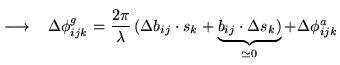
The baseline parameters can be obtained to high accuracy from observations of a number ![]() of relatively strong point sources, well-distributed in hour-angle and declination, for
which accurate positions are available. The analysis of these observations is usually
carried out with CLIC, the calibration program, using a least-square-fit analysis on the
geometric phase difference for antenna pairs (
of relatively strong point sources, well-distributed in hour-angle and declination, for
which accurate positions are available. The analysis of these observations is usually
carried out with CLIC, the calibration program, using a least-square-fit analysis on the
geometric phase difference for antenna pairs (![]() ):
):
In theory, three sources are sufficient to measure the actual baseline lengths, in
practice 10-12 sources are necessary to obtain an accurate measurement. Since a
displacement by 1![]() at 100GHz on a baseline of 100m translates already to a phase
offset of
at 100GHz on a baseline of 100m translates already to a phase
offset of
![]() (
(![]() rad), the positions of the radio sources used for
baseline measurements need to be known with an accuracy
rad), the positions of the radio sources used for
baseline measurements need to be known with an accuracy
![]() better than
better than ![]() .
.
The baseline equation implies that positional errors are equivalent to phase errors. Since baseline length errors scale with the angular separation between calibrator and source, the aim is to have calibrators as close as possible to minimize the phase errors.
Sometimes, accurate baselines are not required as in the case of self-calibration projects. Sometimes, however, even if good baselines are required, they simply cannot be determined precisely enough after a change of configuration. Projects observed in the meantime will then need to wait for a better baseline model. Such projects will in general not be phase-calibrated by the astronomer on duty, but phase-calibration has to be done later on by the proposers of the observations.
Gain measurements (GAIN scans) are cross-correlations on strong radio sources which are essentially used to measure the image to signal sideband ratios for both the 3mm and 1.3mm receivers. The required sideband ratio depends on the project, the achievable sideband ratio depends on the receiver and the frequency. An accurate measurement of the receiver gain is necessary for a good estimate of the atmospheric opacity and of the associated thermal noise with which the atmosphere contributes during the observations.
Therefore, results of a gain measurement are followed by an atmospheric calibration (scan CALI).
As a rule, a high receiver stability
![]() is never
required. Sometimes, however, depending on atmospheric conditions,
array configuration and observing frequency, a higher stability
may be desirable in view of a very promising radiometric phase
correction. Though such a high stability is not always achievable
on all the receivers, it makes possible an improvement in data
quality when the atmospheric phase correction technique becomes
practical (see Chapter 11 by M.Bremer). Experience at
Bure from the last three years shows that the radiometric phase
correction is quite efficient under clear sky conditions: from
spring to autumn essentially during the evening and morning hours,
in winter almost always when the weather allows to observe.
is never
required. Sometimes, however, depending on atmospheric conditions,
array configuration and observing frequency, a higher stability
may be desirable in view of a very promising radiometric phase
correction. Though such a high stability is not always achievable
on all the receivers, it makes possible an improvement in data
quality when the atmospheric phase correction technique becomes
practical (see Chapter 11 by M.Bremer). Experience at
Bure from the last three years shows that the radiometric phase
correction is quite efficient under clear sky conditions: from
spring to autumn essentially during the evening and morning hours,
in winter almost always when the weather allows to observe.
Since observations on more compact baselines suffer less from the effects of the
atmospheric phase noise - for reference, an rms of less than 10![]() rms at 3mm is
routinely obtained on the shortest baselines - a high receiver stability in compact
configurations is only exceptionally required. Typically, under average observing
conditions with a receiver stability of 3.10
rms at 3mm is
routinely obtained on the shortest baselines - a high receiver stability in compact
configurations is only exceptionally required. Typically, under average observing
conditions with a receiver stability of 3.10![]() we may already correct atmospheric
phase fluctuations with a precision of 10
we may already correct atmospheric
phase fluctuations with a precision of 10![]() at 115GHz.
at 115GHz.
Since projects are spread over typically a few months, it is impractical that astronomers actually come to the interferometer for their observations. In some exceptional case, however, when observations require rapid decisions, the presence of a visiting astronomer may become necessary. Up to now and after ten years of operation, only a handful of projects required the presence of a visiting astronomer. Only non-standard observations like mapping of fast moving objects, coordinated observations may require a member of the project team to be present on the site. All observations are currently carried out ``in absentee'', and a local contact is assigned to each project.
The observer has to specify all aspects of his/her program in an observing procedure. For routine observations, this is usually done with the help of the local contact by parameterizing the general observational procedure. Once the procedure is written, a copy is made available to the operation center at Plateau de Bure. Before start, further verifications will be made by the scientific coordinator and, to finalize the procedure, by the astronomer on-duty who makes a last check by looking at the technical details in the proposal, at the technical report and at the recommendations made by the programme committee.
Quite some time, however, may pass between the preparation of an observational procedure and the actual observations. Depending on the requirements, between a few hours and a few months may go for the decision to start the observations. On average 90% of the projects are completed within 6 months from their acceptance.
For the observations, the array is operated by an operator with the assistance of an astronomer and under the supervision of the scientific coordinator. The operator has the full responsibility for conducting all observations following pre-established observing procedures or with the help of the astronomer in case of unpredicted events.
The operator will execute the observing procedure according to a pre-established planning which allows for some flexibility in the scheduling, and to a few criteria (as the maximum amount of precipitable water in the atmosphere, the required atmospheric phase stability, the requested observing frequencies, the declination of the targets, the sun avoidance limit and a few other aspects) which will help both the operator and the astronomer in their final decision-making on which project to carry out as next. As a rule, excellent atmospheric conditions will be used for high grade projects requesting sensitivity at high frequencies while the remaining time will in general be devoted to projects which require less stringent atmospheric conditions.
Once a project is selected, the operator will start the observing procedure which sets up the needed equipment configuration (essentially sky frequencies, correlator settings and target coordinates according with the observer's wishes) and will start preparing the interferometer for the observations: the receivers are tuned, the gains and the zero-delay of the receiving antenna is adjusted and verified, the antenna pointed and focused, the RF passband is measured and the temperature scale of the interferometer calibrated. The flux of the primary calibrators are then verified, eventually replaced if their flux density has dropped too much, and the observations started.
As soon a project is started, the astronomer on-duty will monitor the execution of the project and the data quality by examining the visibility amplitude and phase of the calibration sources, the antenna tracking in presence of wind, the antenna pointing corrections, and all time-dependent instrumental and atmospheric parameters which could have some implications on the observations. Furthermore, to avoid further observing on a target with wrong coordinates, the astronomer will verify the presence or absence of line and/or continuum emission according to the expected values quoted in the proposal. Finally, the astronomer on-duty will provide pre-calibrated data on a best effort basis. Depending on project complexity and needs, further data analysis is sometimes required on the site to decide on follow-up observations.
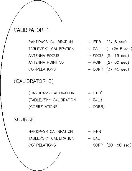 |
When the observations are running, commands are regularly issued to the antennas and to the peripheral equipment (phase rotators, correlators and others) following a well-defined, cyclic sequence as shown in Figure 8.2. This sequence may slightly change depending on the number of calibrators and on the number of phase centers (i.e. the fields of view requested for different sources or for mosaic-type observations) the observer wishes to track in a single run. Typical observations at Plateau de Bure fall in one of the following categories:
Under normal circumstances only a few parameters of interest are regularly verified and corrected (mostly automatically) during the observations, but instantaneous (every second) and much more detailed information can be obtained at any time by connecting to the equipment (receivers, antenna control parameters, digital correlator units and others). During the operation the array status is continuously monitored so that the operator can provide fast feedback in response, at any time when necessary. An automatic data quality assessments (flagging bad data, antenna shadowing, receiver phase lock and others) before writing data to disk. The astronomer on-duty has the responsibility of periodically monitoring the data acquisition and to write a few notes assessing the data quality during and after the observations. Monitoring the progress of a project by making intermediate data reductions, however, is the responsibility of the observer. This is not the responsibility neither of the astronomer on-duty nor of his/her local contact.
 |