Due to space constraints in this book we cannot provide a very detailed overview of all aspects involved in modeling the longwave atmospheric spectrum. The author and co-workers have recently published an in-depth description of their radiative transfer model ATM (Atmospheric Transmission at Microwaves, Pardo et al [2001b]) that can serve as a reference for the information that is missing here. That model has been adopted in this chapter.
We will see in this chapter how to model the Earth's atmosphere longwave spectrum. For millimeter and submillimeter astronomy applications we need to know for a given path through the atmosphere, the opacity, radiance, phase delay and polarization10.1.
The unpolarized radiative transfer in non-scattering media is described by a relatively simple differential scalar equation:
After rearranging equation 10.12 and
considering absence of scattering, the radiative transfer problem
is unidimensional in the direction of ![]() . We can formulate
it under Local Thermal Equilibrium (LTE)
conditions as follows:
. We can formulate
it under Local Thermal Equilibrium (LTE)
conditions as follows:
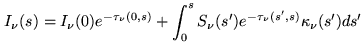
The solution of this equation can be given in an integral form:
In general, the line-by-line integrated opacity corresponding to a path through the terrestrial atmosphere is calculated in a discrete way as follows:
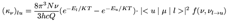
The absorption coefficient of an electric dipole (E1) resonance in the atmosphere is given in general by the following equation:
Both transition probabilities
![]() and
rotational energy levels (from which both resonance
frequencies and population factors under LTE are determined) can
be obtained from the rotational hamiltonians. The number of
rotational constants depends on the type of molecule. The cases
to be considered in the atmosphere are diatomic or
linear molecules (with no magnetic moment), symmetric
rotors in
and
rotational energy levels (from which both resonance
frequencies and population factors under LTE are determined) can
be obtained from the rotational hamiltonians. The number of
rotational constants depends on the type of molecule. The cases
to be considered in the atmosphere are diatomic or
linear molecules (with no magnetic moment), symmetric
rotors in
![]() electronic state, and asymmetric rotors.
electronic state, and asymmetric rotors.
Analytical expressions (see Pardo et al [2001b]) can be used in the atmosphere for both types of molecules within an error not larger than 0.4%.
Of the major molecular constituents of the atmosphere (see
Table 10.1) only water vapor
and ozone, owing to their bent structure,
have a non-zero electric dipole moment. Molecular nitrogen, an
homonuclear species, and CO![]() , a linear symmetric species, have
no permanent electric or magnetic
dipole moment in their lowest energy states. These
latter molecules, as is the case
for most of gaseous molecules, are singlet states, with electrons arranged
two-by-two with opposite spins. O
, a linear symmetric species, have
no permanent electric or magnetic
dipole moment in their lowest energy states. These
latter molecules, as is the case
for most of gaseous molecules, are singlet states, with electrons arranged
two-by-two with opposite spins. O![]() has a permanent magnetic dipole owing to
two parallel electron spins. It thus presents magnetic dipole transitions of
noticeably intensity due to the large abundance of this molecule in the
atmosphere.
has a permanent magnetic dipole owing to
two parallel electron spins. It thus presents magnetic dipole transitions of
noticeably intensity due to the large abundance of this molecule in the
atmosphere.
We present here the details about the spectroscopy of H![]() O, O
O, O![]() and
O
and
O![]() because these molecules dominate the longwave atmospheric spectrum
as seen from the ground.
because these molecules dominate the longwave atmospheric spectrum
as seen from the ground.
For ![]() H
H![]() O each level is denoted, as usual
for asymmetric top molecules by three number s
O each level is denoted, as usual
for asymmetric top molecules by three number s
![]() .
. ![]() , which is a ``good'' quantum number,
represents the total
angular momentum of the molecule; by analogy with symmetric tops,
, which is a ``good'' quantum number,
represents the total
angular momentum of the molecule; by analogy with symmetric tops, ![]() and
and
![]() stand for the rotational angular momenta around the axis of least and
greatest inertia. Allowed radiative transitions obey the selection rules
stand for the rotational angular momenta around the axis of least and
greatest inertia. Allowed radiative transitions obey the selection rules
![]() with
with
![]() or
or
![]() . The levels with
. The levels with ![]() and
and ![]() of the
same parity belong to the para species, those of opposite parity belong
to orto water.
of the
same parity belong to the para species, those of opposite parity belong
to orto water.
Molecular oxygen, although homonuclear, hence with zero electric dipole
moment, has a triplet electronic ground state, with two electrons
paired with parallel spins. The resulting electronic spin couples efficiently with
the magnetic fields caused by the end-over-end rotation of the molecule,
yielding a magnetic dipole moment of two Böhr magnetons,
![]() =2
=2
![]() =1.854
=1.854![]() 10
10![]() Debyes.
The magnetic dipole transitions of O
Debyes.
The magnetic dipole transitions of O![]() have intrinsic strengths
have intrinsic strengths
![]() times weaker than the water transitions. O
times weaker than the water transitions. O![]() , however, is
10
, however, is
10![]() times more abundant than H
times more abundant than H![]() O, so that the atmospheric lines of
the two species have comparable intensities.
O, so that the atmospheric lines of
the two species have comparable intensities.
The spin of 1 makes of the ground electronic state of O![]() a triplet state
(
a triplet state
(![]() ). N, the rotational angular momentum couples with S, the
electronic spin, to give J the total angular momentum: N +S = J. The N
). N, the rotational angular momentum couples with S, the
electronic spin, to give J the total angular momentum: N +S = J. The N![]() S interaction (and the electronic angular
momentum-electronic spin interaction L
S interaction (and the electronic angular
momentum-electronic spin interaction L![]() S) split each rotational level
of rotational quantum number
S) split each rotational level
of rotational quantum number ![]() into three sublevels with total quantum
numbers
into three sublevels with total quantum
numbers
The magnetic dipole transitions obey the rules
![]() and
and
![]() . Transitions within the fine structure sublevels of a rotational level
(i.e.
. Transitions within the fine structure sublevels of a rotational level
(i.e.
![]() ) are thus allowed. The first such transition is the
) are thus allowed. The first such transition is the
![]() transition, which has a frequency of 118.75 GHz. The second, the
transition, which has a frequency of 118.75 GHz. The second, the
![]() transition, has a frequency of 56.26 GHz. It is surrounded by a
forest of other fine structure transitions with frequencies ranging from 53 GHz to
66 GHz. The first "true" rotational transition, the
transition, has a frequency of 56.26 GHz. It is surrounded by a
forest of other fine structure transitions with frequencies ranging from 53 GHz to
66 GHz. The first "true" rotational transition, the
![]() transitions,
have frequencies above 368 GHz (368.5, 424.8, and 487.3 GHz). In addition, the permanent
magnetic dipole of this molecule can interact with an external magnetic field, leading
to a Zeeman splitting of the energy levels. In our atmosphere this splitting is of the
order of 1-2 MHz.
transitions,
have frequencies above 368 GHz (368.5, 424.8, and 487.3 GHz). In addition, the permanent
magnetic dipole of this molecule can interact with an external magnetic field, leading
to a Zeeman splitting of the energy levels. In our atmosphere this splitting is of the
order of 1-2 MHz.
The rare isotopomer ![]() O
O![]() O is not homonuclear, hence has odd
O is not homonuclear, hence has odd
![]() levels and a non-zero electric dipole moment. This latter, however,
is vanishingly small (10
levels and a non-zero electric dipole moment. This latter, however,
is vanishingly small (10![]() D).
D).
The quantum numbers are as in other asymmetric top molecules, such as H![]() O.
As noted above, ozone is mostly concentrated between 11 and 40 km altitude; it shows
large seasonal and, mostly, latitude variation. Because of its high altitude
location, its lines are narrow: at 25 km,
O.
As noted above, ozone is mostly concentrated between 11 and 40 km altitude; it shows
large seasonal and, mostly, latitude variation. Because of its high altitude
location, its lines are narrow: at 25 km, ![]() , hence
, hence ![]() , is reduced by
a factor of 20 with respect to see level; moreover, the dipole moment of ozone
(
, is reduced by
a factor of 20 with respect to see level; moreover, the dipole moment of ozone
(![]() = 0.53 Debyes), 3.5 times smaller than that of H
= 0.53 Debyes), 3.5 times smaller than that of H![]() O, further reduces the ozone
line widths. Because of their small widths and despite the small ozone abundance,
ozone lines have significant peak opacities, especially as frequency increases. This
fact can be seen in the high resolution FTS measurements presented in this chapter.
O, further reduces the ozone
line widths. Because of their small widths and despite the small ozone abundance,
ozone lines have significant peak opacities, especially as frequency increases. This
fact can be seen in the high resolution FTS measurements presented in this chapter.
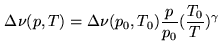
In the lower atmospheric layers (up to ![]() 50 km, depending on
the molecule and the criteria) the collisional broadening
mechanism (also called pressure-broadening) dominates the line
shape. One approximation to the problem considers that the time
between collisions,
50 km, depending on
the molecule and the criteria) the collisional broadening
mechanism (also called pressure-broadening) dominates the line
shape. One approximation to the problem considers that the time
between collisions,
![]() (
(![]()
![]() ), is much
shorter than the time for spontaneous emission,
), is much
shorter than the time for spontaneous emission,
![]() ,
which is, in the case of a two level system, 1/A
,
which is, in the case of a two level system, 1/A
![]() where A
where A
![]() is the Einstein's coefficient for
spontaneous emission. This approximation leads to the so-called
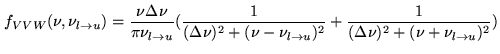
Van Vleck & Weisskopf profile, normalized as follows to be
included in equation 10.16:
is the Einstein's coefficient for
spontaneous emission. This approximation leads to the so-called
Van Vleck & Weisskopf profile, normalized as follows to be
included in equation 10.16:
This lineshape describes quite well the resonant absorption in the
lower atmospheric layers
except for very large shifts from the line centers. For example,
all the mm/submm resonances of
H![]() O and other molecules up to 1.2 THz are well reproduced
using this approximation within that frequency range.
Some properties of the collision
broadening parameters in the atmosphere are:
O and other molecules up to 1.2 THz are well reproduced
using this approximation within that frequency range.
Some properties of the collision
broadening parameters in the atmosphere are:
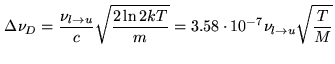
When the pressure gets very low the Doppler effect due to the random thermal molecular motion dominates the line broadening:
![$\displaystyle {\cal{F}}_{D}(\nu,\nu_{l\rightarrow u})=\frac{1}{\Delta \nu_{D}}(...
...2}{\pi})^{1/2} exp[-(\frac{\nu-\nu_{l\rightarrow u}}{\Delta \nu_{D}})^{2}\ln 2]$](img1187.png) |
(10.20) |
 |
(10.21) |
If the collisional and thermal broadening mechanisms are comparable the resulting line-shape is the convolution of a Lorentzian (collisional line shape at low pressures) with a Gaussian: a Voigt profile.
Besides absorption, the propagation through the atmosphere also introduces a phase delay. This phase delay increases as the wavelength approaches a molecular resonance, with a sign change across the resonance. The process can be understood as a forward scattering by the molecular medium in which the phase of the radiation changes.
Both the absorption coefficient and the phase delay
can be treated in a unified way for any system since both
parameters are derived from a more fundamental property,
the complex dielectric constant, by means of
the Kramers-Krönig
relations. A generalized (complex) expression of the VVW
profile, which accounts for both the
Kramers-Krönig
dispersion theory as well as line overlapping
effects (parameter ![]() ) is the
following (
) is the
following (
![]() ):
):
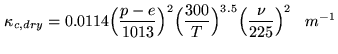
The non resonant absorption of the dry atmosphere is made
up of two components: collision induced absorption due to
transient electric
dipole moments generated in binary interactions
of symmetric molecules with electric quadrupole moments
such as N![]() and O
and O![]() , and the relaxation (Debye) absorption
of O
, and the relaxation (Debye) absorption
of O![]() .
.
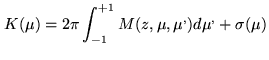
The equation describing the transfer of radiation through an atmosphere that contains scatterers is as follows:
 |
![]() ,
, ![]() and
and ![]() are related according to:
are related according to:
The frequency independent (excluding Raman effect or fluorescence) far-field scattering by single non-spherical particles has been incorporated to the ATM model. It is computed using state-of-the-art T-Matrix routines developed by Mishchenko [2000]. For the integration over all possible orientations to be possible, it is necessary to be in the single scattering regime. Then, each particle is in the far-field zone of the others. This implies that the average distance between particle centers is larger than 4 times their radii. This requirement is usually satisfied by cloud and precipitation particles. The scattered fields are then incoherent and their Stokes parameters can simply be added.
For estimates concerning the effect of clouds to ground-based observations a plane parallel geometry is assumed, as a first approach, with thermal emission as the only source of radiation. The hydrometeors can be either totally randomly-oriented or at least azimuthally randomly oriented. In both cases, the radiation field is azimuthally symmetric leading the Stokes parameters U and V to vanish so that the dimension of tensorial equation (10.25) reduces to be 2. This radiative transfer equation can then be integrated using the quite standard method called doubling and adding, introduced in the ATM model according to Evans & Stephens [1991].
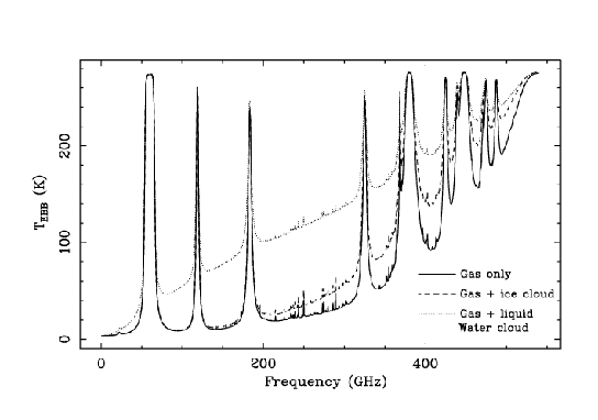
To illustrate the effect of two different types of clouds, we have
performed first a simulation where we add to a clear atmosphere
containing 1 mm of water vapor a layer between 6 and 6.5 km that
contains spherical water droplets with a radius of 40 ![]() m and
a liquid water path of 0.1 km/m
m and
a liquid water path of 0.1 km/m![]() . The second simulation
replaces the water droplets for spherical ice particles with a
radius of 100
. The second simulation
replaces the water droplets for spherical ice particles with a
radius of 100 ![]() m. The effect of liquid water is
quite large since it is a quite effective absorber. The
effect of ice is much more related with its scattering
properties and becomes more important at shorter wavelengths.
m. The effect of liquid water is
quite large since it is a quite effective absorber. The
effect of ice is much more related with its scattering
properties and becomes more important at shorter wavelengths.
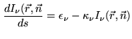
![$\displaystyle \frac{dI_{\nu}(s')}{d\tau_{\nu}}=-I_{\nu}(s')+S_{\nu}(T[s'])$](img1118.png)
![$\displaystyle \tau_{\nu}(s',s)=\sum_{i(layers)}^{}[\sum_{j(molec.)}^{ } (\sum_{k(resonances)}^{ } \kappa_{\nu_{k}})_{j}]_{i}\cdot \Delta s_{i}$](img1123.png)
![$\displaystyle {\cal{F}}_{VVW}(\nu,\nu_{lu})=\frac{\nu}{\pi \nu_{lu}} [\frac{1-i\delta}{\nu_{lu}-\nu-i\Delta \nu} +\frac{1+i\delta}{\nu_{lu}+\nu+i\Delta \nu}]$](img1190.png)
![$\displaystyle \kappa_{c,H_{2}O}=0.031\cdot\Bigl(\frac{\nu}{225}\Bigr)^{2} \cdot...
...1013}\cdot\frac{p-e}{1013}\Bigr]\cdot \Bigl(\frac{300}{T}\Bigr)^{3}\;\;\;m^{-1}$](img1192.png)
![$\displaystyle \mu\frac{dI(z,\mu)}{dz}={K} (z,\mu)I(z,\mu) -2\pi\int_{-1}^{1}M(z,\mu,\mu') I(z,\mu')d\mu'-\sigma(z,\mu)B[T(z)]$](img1194.png)