1.2 Basic Principles

The properties of electromagnetic radiation propagation and of radio antennas can be deduced from a few basic physical principles, i.e.

1. the notion that Electromagnetic Radiation are Waves of a certain Wavelength ($\lambda$), or Frequency ($\nu$), and Amplitude (A) and Phase ($\varphi$);
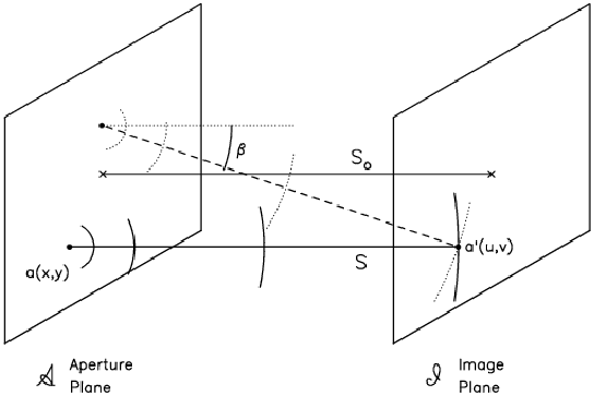
2. from Huygens Principle which says that each element of a wavefront is the origin of a Secondary Spherical Wavelet;
3. the notion that the Optical Instrument (like a single-dish antenna, a telescope, etc.) combined with a receiver manipulates the incident wavefront through their respective phase and amplitude transfer functions.

$\parbox{120mm}{ \caption{ Illustration ... ... optical instrument (telescope) is placed in between $\cal A$ and $\cal I$. }}$

Summarized in one sentence, and proven in the following, we may say that the radio antenna transforms the radiation incident on the aperture plane ($\cal A$) to an image in the image plane ($\cal I$), also called focal plane. Following Huygens Principle illustrated in Figure 1.1, the point a(x,y) $\equiv$ a($\vec r$) of the incident wavefront in the aperture plane $\cal A$ is the origin of a spherical wavelet of which the field $\delta$E(a$'$) at the point a$'$(u,v) $\equiv$ a($\vec u$) in the image plane $\cal I$ is

$${\delta}{\rm E}({\vec u}) = {\rm A}({\vec r}){\rm exp[iks]/s}$$ (1.1)

with k = 2 $\pi/\lambda$. The ensemble of spherical wavelets arriving from all points of $\cal A$ at the point a$'(\vec u)$ of the image plane $\cal I$ produces the field

$${\rm E}({\vec u}) = {\int}_{{\cal A}}{\rm A}({\vec r}){\Lambda}({\beta}) [{\rm exp(iks)/s}] dx dy$$ (1.2)

For the paraxial case, when the rays are not strongly inclined against the direction of wave propagation (i.e. the optical axis), the inclination factor $\Lambda$ can be neglected since $\Lambda$($\beta$) $\approx$ cos($\beta$) $\approx$ 1. Also, s $\approx$ s$_{0}$ for paraxial rays, but exp[iks] $\neq$ exp[iks$_{0}$] since these are cosine and sine terms of s where a small change in s may produce a large change of the cosine or sine value. Thus, for the paraxial approximation we may write

$$s = [{\rm (x-u)}^2 + {\rm (y-v)}^2 + {\rm z}^2]^{1/2} \approx {\rm R + g(x,y,R) - (xu + yv)/R}$$ (1.3)

with

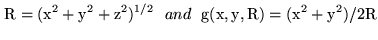$${\rm R} = ({\rm x}^2 + {\rm y}^2 + {\rm z}^2)^{1/2} and {\rm g(x,y,R)} = ({\rm x}^2 + {\rm y}^2)/2{\rm R}$$ (1.4)

When using these expressions in Eq.1.2, we obtain

$${\rm E(u,v) = [exp(ikR)/s}_{0}]{\int}_{{\cal A}}{\rm A(x,y)} {\rm exp[ik(g(x,y,R) - (ux + vy)/R)] dx dy}$$ (1.5)

This equation describes the paraxial propagation of a wavefront, for instance the wavefront arriving from a very far away star. In particular, this equation says, that without disturbances or manipulations in between $\cal A$ and $\cal I$ the plane wavefront continues to propagate in straight direction as a plane wavefront.