We now place an optical instrument (a mirror, lens, telescope etc.) in the beam
between ![]() and
and ![]() with the intention, for instance, to form an image of
a star. Optical instruments are invented and developed already since several
centuries; however, the physical-optics (diffraction) understanding of the image
formation started only a good 200 years ago. Thus, speaking in mathematical terms,
the telescope (T) manipulates the phases (not so much the amplitudes) between the
points (
with the intention, for instance, to form an image of
a star. Optical instruments are invented and developed already since several
centuries; however, the physical-optics (diffraction) understanding of the image
formation started only a good 200 years ago. Thus, speaking in mathematical terms,
the telescope (T) manipulates the phases (not so much the amplitudes) between the
points (![]() ) of the aperture plane (
) of the aperture plane (![]() ) and the points (
) and the points (![]() ) of the
image plane (
) of the
image plane (![]() ) by the phase transfer function
) by the phase transfer function
![]() , so that the wavefront converges in the focal point. The
receiver(R)/detector introduces an additional modulation of the amplitude
, so that the wavefront converges in the focal point. The
receiver(R)/detector introduces an additional modulation of the amplitude
![]() , as described below. Using this information, the
field distribution in the focal plane (
, as described below. Using this information, the
field distribution in the focal plane (![]() ) of the telescope becomes
) of the telescope becomes
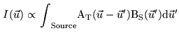
This equation says that the field distribution E(![]() ) in the
focal plane of the telescope is the Fourier transform (
) in the
focal plane of the telescope is the Fourier transform (![]() )
of the receiver-weighted field distribution A(
)
of the receiver-weighted field distribution A(![]() )
)
![]() in the aperture plane. Since E(
in the aperture plane. Since E(![]() )E
)E
![]() for a realistic
optical instrument/telescope with limited aperture size, we
arrive at the well known empirical fact that the image of a
point-like object is not point-like; or; with other words, the
image of a star is always blurred by the beam width of the antenna
for a realistic
optical instrument/telescope with limited aperture size, we
arrive at the well known empirical fact that the image of a
point-like object is not point-like; or; with other words, the
image of a star is always blurred by the beam width of the antenna
![]() , with
, with ![]() the
diameter of the reflector.
the
diameter of the reflector.
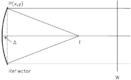
To close the argumentation, we need to show that the telescope manipulates the incident wave in the way given by Eq.1.7). To demonstrate this property in an easy way, we consider in Figure 1.2 the paraxial rays of a parabolic reflector of focal length F. From geometrical arguments we have
| (1.9) |
| (1.10) |
The fundamental Eq.1.8 can be used to show that an interferometer is not a single dish antenna, even though one tries with many individual telescopes
and many telescope positions (baselines) to simulate as good as possible the
aperture of a large reflector. If we assume for the single dish antennas that
A(
![]() and
and
![]() , then the power pattern P(
, then the power pattern P(![]() ) (beam pattern) in the focal plane of the single antenna is
) (beam pattern) in the focal plane of the single antenna is
![$\displaystyle {\rm P}({\vec u}) = {\rm E}({\vec u}){\rm E}^{*}({\vec u}) = {\in...
...(dxdy)}_{1}{\rm (dxdy)}_{2} {\propto} [{\rm J}_{1}({\vec u})/{\rm u}]^{2}$](img164.png) |
(1.11) |
where J![]() is the Bessel function of first order (see
[Born & Wolf 1975]). The function [J
is the Bessel function of first order (see
[Born & Wolf 1975]). The function [J![]() (u)/u]
(u)/u]![]() is called Airy
function, or Airy pattern. The interferometer does not simulate a
continuous surface, but consists of individual aperture sections
is called Airy
function, or Airy pattern. The interferometer does not simulate a
continuous surface, but consists of individual aperture sections
![]() ,
,
![]() , .... of the individual telescopes, so
that its power pattern P
, .... of the individual telescopes, so
that its power pattern P
![]() ) (beam pattern) in the
focal plane is
) (beam pattern) in the
focal plane is
![$\displaystyle {\rm P}_{\Sigma}({\vec u}) = {\sum}_{\rm n}{\sum}_{\rm m}{\int}_{...
... {\vec x}_{2})] {\rm (dxdy)}_{1}{\rm (dxdy)}_{2} {\neq} {\rm P}({\vec u})$](img168.png) |
(1.12) |
The single telescope selects a part of the incident plane wavefront and 'bends' this
plane into a spherical wave which converges toward the focus. This spherical
wavefront enters the receiver where it is mixed, down-converted in frequency,
amplified, detected, or correlated. The horn-lens combination of the receiver
modifies the amplitude of the spherical wavefront in a way expressed by the function
![]() . This function, called taper or illumination function of
the horn-lens combination, weighs the wavefront across the aperture, usually in a
radial symmetric way. Figure 1.3 shows, schematically, the effect of a
parabolic taper as often applied on radio telescopes, and expressed as
. This function, called taper or illumination function of
the horn-lens combination, weighs the wavefront across the aperture, usually in a
radial symmetric way. Figure 1.3 shows, schematically, the effect of a
parabolic taper as often applied on radio telescopes, and expressed as
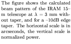
Figure 1.4 shows as example a two-dimensional cut through the calculated
beam pattern A![]() of the IRAM 15-m telescope at
of the IRAM 15-m telescope at ![]() = 3mm, once
without taper (i.e. for
= 3mm, once
without taper (i.e. for
![]() ), and for a -10 dB edge
taper, i.e. when the weighting of the wavefront at the edge of the aperture is 1/10
of that at the center (see Figure 1.3). As seen from the figure, the taper
preserves the global structure of the non-tapered beam pattern, i.e. the main beam
and side lobes, but changes the width of the beam (BW:
), and for a -10 dB edge
taper, i.e. when the weighting of the wavefront at the edge of the aperture is 1/10
of that at the center (see Figure 1.3). As seen from the figure, the taper
preserves the global structure of the non-tapered beam pattern, i.e. the main beam
and side lobes, but changes the width of the beam (BW:
![]() ), the
position of the first null (
), the
position of the first null (
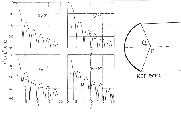
![]() ), and the level of the side lobes. The
effect of the taper depends on the steepness of the main reflector used in the
telescope, as shown in Figure 1.5. The influence of several taper forms is
given in Table 1.1 [Christiansen and Hogbom 1969].
), and the level of the side lobes. The
effect of the taper depends on the steepness of the main reflector used in the
telescope, as shown in Figure 1.5. The influence of several taper forms is
given in Table 1.1 [Christiansen and Hogbom 1969].
|
The complete telescope, i.e. the optics combined with the receiver, has a beam
pattern A
![]() (in optics called point-spread-function) with which we
observe point-like or extended objects in the sky with the intention to know their
position, structural detail, and brightness distribution B
(in optics called point-spread-function) with which we
observe point-like or extended objects in the sky with the intention to know their
position, structural detail, and brightness distribution B![]() as function of
wavelength. The telescope thus provides information of the form
as function of
wavelength. The telescope thus provides information of the form
 |
(1.15) |
When we point the antenna toward the sky, in essence we point the beam in the
direction of observation. If, for instance, we observe a point-like source it is
evident that the peak of the main beam should point exactly on the source which
requires that the pointing errors (
![]() ) of the telescope should be small
in comparison to the beam width. The loss in gain is small, and acceptable, if the
mispointing
) of the telescope should be small
in comparison to the beam width. The loss in gain is small, and acceptable, if the
mispointing
![]() . Since modern radio telescopes use
an alt-azimuth mount, this criterion says the mispointing in azimuth
(
. Since modern radio telescopes use
an alt-azimuth mount, this criterion says the mispointing in azimuth
(
![]() ) and elevation (
) and elevation (
![]() ) direction should
not exceed 1/
) direction should
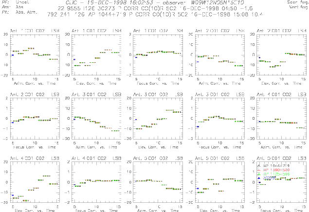
not exceed 1/![]() this value. The pointing and focus (see below) of the IRAM
antennas are regularly checked during an observation, and corrected if required. The
corresponding protocol of an observing session at Plateau de Bure, using 5 antennas,
is shown in Figure 1.6.
this value. The pointing and focus (see below) of the IRAM
antennas are regularly checked during an observation, and corrected if required. The
corresponding protocol of an observing session at Plateau de Bure, using 5 antennas,
is shown in Figure 1.6.
![$\displaystyle {\rm E}({\vec u}) = [{\rm exp(ikR)/s}_0]{\int}_{{\cal A}}{\rm A}(...
...r}){\Omega}_{\rm O} {\Omega}_{\rm R}{\rm exp[ik(g(x,y,R) - (ux + vy)/R)] dx dy}$](img150.png)
![$\displaystyle {\rm E}({\vec u}) = {\rm [exp(ikF)/F]}{\int}_{{\cal A}}{\rm A}({\...
...)/F]dxdy} {\equiv} {\cal FT}[{\rm A}({\vec r}){\Omega}_{\rm R}({\vec r})]$](img152.png)
![\resizebox{8cm}{!}{\includegraphics[angle=0.0]{greve3.eps}}](img173.png)
![\resizebox{8cm}{!}{\includegraphics[angle=0.0]{greve4.eps}}](img180.png)