We have already encountered the effects of atmospheric absorption in the lecture by Michel Guélin (Chapter 10). Even under low opacity conditions, observations can be difficult or impossible due to atmospheric phase fluctuations. In principle, integration of an interferometric signal is like the adding up of vectors. The amplitude is the length of a vector, and its orientation is given by the phase. Errors in the phase will cause part of the amplitudes to cancel each other out according to Eq. 11.1
If our eyes were sensitive in the millimeter range with a resolving power of some arc seconds, we would not only see a luminous sky where sources are difficult to make out on the background: we would notice refracting bubbles of sizes between some centimeters to several kilometers drifting with the wind, merging, separating and distorting the view behind them. It is water vapor which has not attained the concentrations necessary for cloud formation, and mixes badly with dry air. Even in the case of low opacity and a sky clear for human perception, these distortions - which are shifts and tilts in the incoming phase front - can be so important that they make observations impossible.
In this lecture we will study the physics behind this effect and possible ways to correct for it which have become available in recent years.
The phases of a wave front that reaches ground-based observatories have been modified by their journey through refractive index variations in the Earth's atmosphere. The instrument itself has no way to tell which part of the phases are due to valuable structure in the astronomical source and which part was caused during the last kilometers in front of the telescope.
As a result, the apparent position of a point source keeps moving, so that details of an extended source become blurred (``seeing''). The perturbations become progressively decorrelated with increasing separation between two lines of sight.
Depending on turbulence scale, wavelength and telescope size, a ground-based observer will be confronted with different effects. To some extent, one can reduce unwanted perturbations by choosing an observatory's site carefully. But there are always some days which are better than others.
For a small radio telescope, the phase noise passes unnoticed (Fig.11.1).
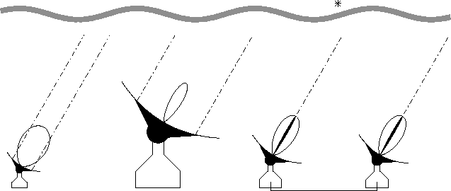 |
The interest of interferometric phase correction is to determine and remove the atmospheric phase noise. Each individual antenna has to correct a time variable ``piston'' in the incoming wave front, which is the equivalent of adaptive optics for the synthesized dish.
Most of the water vapor is confined to the troposphere (![]() 10 km) with an
exponential scale height of 2 km. Its molecular weight is 18.2 g/mol so that it has
the tendency to rise above dry air (28.96 g/mol). Our planet retains the water vapor
due to the negative vertical temperature gradient in the troposphere, and the fact
that H
10 km) with an
exponential scale height of 2 km. Its molecular weight is 18.2 g/mol so that it has
the tendency to rise above dry air (28.96 g/mol). Our planet retains the water vapor
due to the negative vertical temperature gradient in the troposphere, and the fact
that H![]() O is close to the transition points to liquid and solid under terrestrial
pressure and temperature conditions. Venus is an example for a planet with a hot
troposphere (extreme CO
O is close to the transition points to liquid and solid under terrestrial
pressure and temperature conditions. Venus is an example for a planet with a hot
troposphere (extreme CO![]() and H
and H![]() O greenhouse effect) who lost most of its water
long ago.
O greenhouse effect) who lost most of its water
long ago.
Under Earth's environmental conditions, water vapor mixes badly with dry air and tends to form bubbles with sizes up to several kilometers, which are broken up by turbulent motions. When choosing high and dry sites for millimeter astronomy, one must keep in mind that high phase noise can be induced even by low amounts of precipitable water.
Parameters that influence interferometric phase noise strongly are:
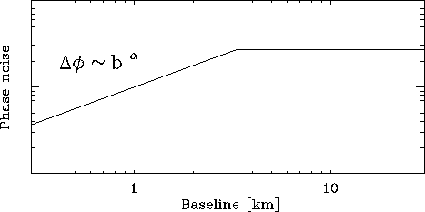 |
The leveling off of the phase noise on a high, constant value corresponds to the outer scale size of the turbulence, where the fluctuations along two lines of sight become totally decorrelated, i.e. as bad as they can possibly get (Fig. 11.2). Increasing the baselines will not increase the phase noise any more, and this is why very long baseline interferometry can work.
In the following, some fundamentals about turbulence will be explained, and how one can analyze the properties of a turbulent atmosphere. Possible methods to monitor the phase fluctuations will be discussed, with emphasis on the phase monitoring system on the Plateau de Bure. Some examples with observational data will be presented, demonstrating its benefits and current limitations.