11.2 Hydrodynamical basics of turbulent motion

Turbulence has its origin in the non-linearities of the hydrodynamical equations of motion. These equations are not derived from first principles, but present the easiest consistent way of describing the motion of compressible (gases) or incompressible (liquids) media. Given the complexity of observed hydrodynamical phenomena (white water rivers, curling smoke, ...) it was doubted for more than a century if the equations could really be as simple as given below.

Scepticism was nourished by the fact that some stationary (i.e. time invariant) solutions were mathematically valid but not observed experimentally, which can be understood today by checking the solutions for their stability. It is an interesting fact that stationary solutions are not always the most stable ones - this assumption might appear ``natural'', but is in fact quite misleading. To find out under which conditions one has to expect turbulence, we must have a closer look into the equations of hydrodynamics.

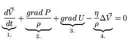
In a free flow (i.e. no outer confinements like tubes) and under sub-sonic conditions, one can treat air as an incompressible medium. This allows to use the Navier-Stokes equations which describe such a medium with viscosity (Eq. 11.2).

$$\underbrace{\frac{d \vec{V}}{d t}}_{1.} + \underbrace{\frac{grad ... ...rbrace{grad \: U}_{3.} - \underbrace{\frac{\eta}{\rho} \Delta \vec{V}}_{4.} = 0$$ (11.2)

The respective terms describe:

1. This part is the complete derivative in time, containing non-linear terms:

   $$\frac{d \vec{V}}{d t} = \frac{\delta \vec{V}}{\delta t} + \left (... ...erbrace{\vec{V} \times \left ( \vec{\nabla} \times \vec{V} \right )}_{Vortices}$$ (11.3)

   
   

2. The pressure term describes the reaction to external forces, and is related to density and temperature through the equation of state.
3. External forces, described by the gradient of a Potential U. This form makes it easier to include this term into the others. We are interested here in cases where $U$ is constant in good approximation, so we can leave this term out in the following.
4. Energy dissipation. Viscous terms, with the Laplacian operator $\Delta = \nabla^2 = div \; grad$ . The material constant $\eta$ is the viscosity coefficient for incompressive media (there is a term with a second coefficient for compressive media, but it can be neglected here).

To solve Equation 11.2, one needs:

• the equation of state for the gas,
• the conservation of mass and energy,
• the boundary conditions.

We will not have to deal with these equations directly. If you have to solve them for some reason: There is a whole class of numerical methods and library codes in the literature, which avoid non-evident pitfalls concerning different coordinate systems and numerical stability. For the current discussion, we are only interested in the question of similarity.

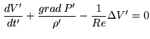
Flow problems resemble each other for certain combinations of flow velocity, spatial dimension and viscosity. This allows to predict the general properties of a hydrodynamic system (and if it is turbulent or not) from small models or other well-studied cases where the geometries are the same. It is convenient to change to dimensionless equations by expressing lengths and velocities in units of the system's typical length scale $l_0$ (e.g. the size of an obstacle) and the unperturbated flow velocity $V_0$.

One obtains not only $V'=V/V_0$ and $l'=l/l_0$, but must change all other units which are combinations of the two: $t'=t\cdot v_0/l_0$, $\rho'=\rho \cdot l_0^3$ and $P'= P \cdot l_0^3/v_0^2$. As a result, we get the dimensionless equation Eq.11.4:

$$\frac{dV'}{dt'}+\frac{grad \: P'}{\rho'}-\frac{1}{Re} \Delta V' = 0$$ (11.4)

which contains Reynold's number $Re = l_0 \cdot V_0 \cdot \rho / \eta$. It determines the relative influence of the energy dissipating term relative to the non-linear turbulent term. A high Reynold's number will reduce the effect of $\Delta V'$, so that turbulence will develop. Each problem has its specific Critical Reynold's number $Re_c$, which lies typically between 10 and 100. For a given geometry and a $Re>Re_c$, no stable solution exists (e.g. Figure 41-6 from [Feynman et al. 1964]).

With Eq.11.4 and the viscosities from Tab.11.1, we find that for ambient conditions, wind moving faster than 1 cm/s hitting an obstacle bigger than 1 cm generates a turbulent flow. A house (10 m) in a 10 m/s wind has $Re\approx 6\cdot 10^6$, mountains $Re\approx 1\cdot 10^9$.

Table 11.1: Examples for viscosity and the kinetic viscosity $\eta /\rho$ various media at 20$^{\circ }$C (adapted from [Landau & Lifshitz 1959]). The viscosity changes little with altitude, so that the density dependency of $\nu$ dominates and satellites above $\approx 300$ km altitude experience a non-turbulent, laminar flow.

Medium	$\eta$ [g/cm s]	$\nu=\eta/\rho$ [cm$^2$/s]
Water	0.010	0.010
Air	0.00018	0.150
Alcohol	0.018	0.022
Glycerin	8.5	6.8
Mercury	0.0156	0.0012

This means that turbulence is something quite common in our environment. In our daily life, we encounter many turbulent systems which defy detailed prediction: leaves of wind-moved trees, eddies in flowing water, the structure of clouds, to name only a few. All these effects are non-linear and will never repeat themselves exactly, although their parameters stay within certain limits.

It may be surprising that these phenomena have been neglected by classical physics for centuries, to become finally popular in the wake of chaos theory and the development of powerful computers. One reason for this was surely the problem of repeating an experiment with inherent chaos exactly, and the sheer bulk of work for doing the calculations. Linear physics were favored not because they are more abundant in nature, but because they were easier to understand and reproduce.

Even chaos theory has a hard time with the atmosphere. The famous ``strange attractors'' which describe non-repetitive curves in solution spaces are not very useful for turbulence, because one is not sure if the number of solution space dimensions is finite or not in this case.

Meteorology is a well-known (and sometimes notorious) example for predictions of a non-linear system. In spite of a network of measurement stations and satellite data, boundary conditions are not known precisely enough for long term forecasts. This is the famous ``butterfly effect'': A butterfly moving its wings in South America may change the weather in Europe six months later.

But don't start hunting butterflys to prevent storms right now: this example only illustrates that non-linear systems do not obey the ``small cause - small effect'' rule of linear physics but a rather imprecise ``small cause at the right place may have a big effect'' rule. So it could be a butterfly, a spoken word, a thought, or a tree falling in a forest, or all of them together that may tip a balance.

For all practical applications, the interactions are too complex to backtrack the cause - but nevertheless, the history that makes a leaf move right now in a unique way outside your window contains somewhere the gravitational pull of faraway galaxies, and your mere presence will leave traces in the turbulent structures all over the universe (no liabilities implied, fortunately).

A small perturbation may set off a non-linear cause-and-effect chain, but this is only because a turbulent system can have multiple macroscopically different states without violating the conservation of energy. Using a statistical approach, we will now discuss turbulence's energy distribution on different scale sizes. This is an important step to understand how atmospheric parameters (including phase noise) change with time and distance.