We start with a simple model of turbulence. It must explain why
the scale size of the finest turbulence structures becomes smaller
and smaller with increasing ![]() , and should allow to treat the
finest details in a homogeneous way. It cannot explain why certain
structures form and not others, but it describes the average flow
of energy across the scale sizes of turbulence.
, and should allow to treat the
finest details in a homogeneous way. It cannot explain why certain
structures form and not others, but it describes the average flow
of energy across the scale sizes of turbulence.
The inertia range is interesting for us because it corresponds to spatial dimensions of some meters to 2-3 kilometers, i.e. the baselines of the PdBI fall into this range.
For the mathematical treatment of highly developed turbulence, one can use a formalism based on random variations.
Most ``classical'' statistics represent a given distribution of probability (binomial, Poisson, Gaussian, ...) around a most likely measurement value. For atmospheric parameters like e.g. temperature and wind velocity, we must make a more general approach: the most likely measurement values vary with time and space, which means they can be represented by non-stationary random processes. The classical average and its variation are not very useful to describe these systems.
An instrument for the characterization of non-stationary random variables are structure functions, which were first introduced by [Kolmogorov 1941]. A scalar structure function has the form given in Eq.11.5,
The structure function formalism can even be used to describe vector parameters like
the turbulent wind velocity, in this case one simply needs
![]() tensors of
structure functions for their description. We won't need tensors in the following
discussion, however. The detailed mathematical formalism of random fields would be
too much for this course (see [Tatarski 1971] for details). We will only discuss
the basic concepts and their application to phase shifts.
tensors of
structure functions for their description. We won't need tensors in the following
discussion, however. The detailed mathematical formalism of random fields would be
too much for this course (see [Tatarski 1971] for details). We will only discuss
the basic concepts and their application to phase shifts.
Real atmospheric parameters are functions of time and space. For time dependency, Taylor's hypothesis of frozen turbulence has been quite successful (Eq.11.6). It states that the pattern of refractive index variations stays fixed while it is moving with the wind.
For two measurement points which are a distance ![]() apart from each other, one finds
that the structure functions of many atmospheric parameters (temperature, refractive
index, absolute wind velocity, ...) obey a
apart from each other, one finds
that the structure functions of many atmospheric parameters (temperature, refractive
index, absolute wind velocity, ...) obey a ![]() power law. This law can be
derived from the theory of random fields, but the easiest way is as follows:
power law. This law can be
derived from the theory of random fields, but the easiest way is as follows:
Consider a velocity fluctuation
![]() (where
(where
![]() may be large)
which occurs on a scale size
may be large)
which occurs on a scale size ![]() and a time
and a time
![]() :
:
| (11.7) |
| (11.8) |
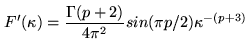
In a thick turbulent layer, the phase front encounters multiple refractive index fluctuations and the power law index changes. This problem can be solved by analyzing the irregular refracting medium over its Fourier transform. After [Tatarski 1961], the spectral density of the function
| (11.9) |
 |
(11.10) |
![$\displaystyle D_{\varphi}(r)=4 \pi \int_0^{\infty}[1-J_0(\kappa r)] F'(\kappa) \kappa d\kappa$](img1334.png) |
(11.11) |
| (11.12) |
Due to the quasi-random nature of phase fluctuations, forecasts and inter/extrapolations can be considered inadequate for a phase correction system. Direct measurements of the water vapor column along the line of sight are therefore the most reliable approach.
 |