All measurements need to be relative to some source of known flux. In practice,
planets are used because they are among the few astronomical objects sufficiently
strong at millimeter wavelengths for which flux density predictions are possible
and sufficiently accurate. They are then used as primary calibrators to bootstrap
the flux of the stronger quasars which are point sources. Since the quasars are
highly variable, a regular monitoring (each month) is needed. These observations
require a very good weather with a small amount of precipitable water vapor
(![]() 4 mm) and a stable atmospheric phase. If not properly taken into account, the
quasar variability can produce an error in the flux scale during one configuration
which does not result in a simple scale factor in the final image, but introduces
artifacts.
4 mm) and a stable atmospheric phase. If not properly taken into account, the
quasar variability can produce an error in the flux scale during one configuration
which does not result in a simple scale factor in the final image, but introduces
artifacts.
Because of the physics of quasars, the spectral index may be variable with time as the source intensity. Simultaneous measurements at 2 frequencies are thus needed to estimate it accurately, IRAM instruments (30-m and PdBI) use the frequencies of 86.7 GHz and 228 GHz. At the 30-m, flux density measurements are done during the pointing sessions while they are performed in special sessions at Bure, usually after baseline measurements.
The results of the flux sessions are regularly reduced and published in an internal report (usually each 4 months). These reports are currently available on the web, in the local IRAM page (see).
In practice, it is impossible (and not necessary) to follow all the quasars used as
amplitude calibrator at the IRAM interferometer. Monitoring of the RF bandpass
calibrators which are strong quasars with flux density ![]() Jy (no more than 4-8
sources) is enough. In the meantime, planets are observed as primary calibrators.
These sessions require to calibrate the atmosphere (
Jy (no more than 4-8
sources) is enough. In the meantime, planets are observed as primary calibrators.
These sessions require to calibrate the atmosphere (![]() ) on each source and to
check regularly the focus.
) on each source and to
check regularly the focus.
At the Bure interferometer, the flux density measurements on quasars are done by
pointings in interferometric mode. Pointings on planets are actually done in total
power mode because they are resolved by interferometry and strong enough. Total
power intensity is not affected by the possible decorrelation due to atmospheric
phase noise. However, it is then necessary to accurately determine the efficiencies
of the individual antennas (conversion factor in Jy/K) in interferometric mode
(
![]() ) and in single-dish mode (
) and in single-dish mode (
![]() ).
).
For each flux session,
![]() is measured on planets by comparison with the models
(see GILDAS programs ASTRO or FLUX).
is measured on planets by comparison with the models
(see GILDAS programs ASTRO or FLUX).
For a given antenna, the interferometric efficiency
![]() is
always
is
always
![]() . Pointing measurements in interferometric
mode are not limited by the atmospheric decorrelation because the
timescale of the atmospheric decorrelation is usually
significantly larger than the time duration of the basic pointing
integration time (
. Pointing measurements in interferometric
mode are not limited by the atmospheric decorrelation because the
timescale of the atmospheric decorrelation is usually
significantly larger than the time duration of the basic pointing
integration time (![]() a few sec). On the contrary, all
instrumental phase noise on very short timescale can introduce a
significant decorrelation and degrades
a few sec). On the contrary, all
instrumental phase noise on very short timescale can introduce a
significant decorrelation and degrades
![]() . This is what may
happen from time to time at a peculiar frequency due to a bad
optimization of the receiver tuning.
. This is what may
happen from time to time at a peculiar frequency due to a bad
optimization of the receiver tuning.
For example, in the initial 1.3mm observations, strong decorrelation was
introduced by the harmonic mixer of the local oscillator system which degraded
![]() by a factor of
by a factor of ![]() depending of the antennas. This problem has been
solved recently. Now at 3mm, it is reasonable to neglect the instrumental noises
and take
depending of the antennas. This problem has been
solved recently. Now at 3mm, it is reasonable to neglect the instrumental noises
and take
![]() . At 1.3mm, the new harmonic mixers have been installed
only recently and statistics on the site are rare but laboratory measurements show
that the loss in efficiency should be small. The Table 12.2 gives the
antenna efficiencies
. At 1.3mm, the new harmonic mixers have been installed
only recently and statistics on the site are rare but laboratory measurements show
that the loss in efficiency should be small. The Table 12.2 gives the
antenna efficiencies
![]() , as measured in flux sessions or by holography.
, as measured in flux sessions or by holography.
|
Being able to cancel out most of the instrumental phase noise even at 1.3mm makes the IRAM interferometer a very reliable instrument. It is reasonable to think that, in the near future, the flux calibration will be systematically performed at Bure at the beginning of each project by reference to the antenna efficiencies. This is indeed already the case: after pointing and focusing, we systematically measure the flux of calibrators when starting a new project (data labeled FLUX in files). Up to now, for typical weather conditions, most (more than 90 %) of the flux measured at 3mm are correct within 10 % and more than 60 % at 1.3mm are within 15 %.
Finally, for each project, a complementary flux check is systematically done using the continuum sources CRL618 or MWC349 (pointing + cross-correlations). However these sources must be used with some caution. CRL618 is partially resolved in A and B configurations at 3mm and in A,B,C at 1.3mm. Moreover it has strong spectral lines which may dominate the average continuum flux; this must be checked before using it for flux estimates. MWC349 is unresolved and remains a reliable reference in all antenna configurations. The only strong lines for MWC349 are the Hydrogen recombination lines. The adopted flux densities are:
For CRL618 (see flux reports 13 and 15):
For MWC349:
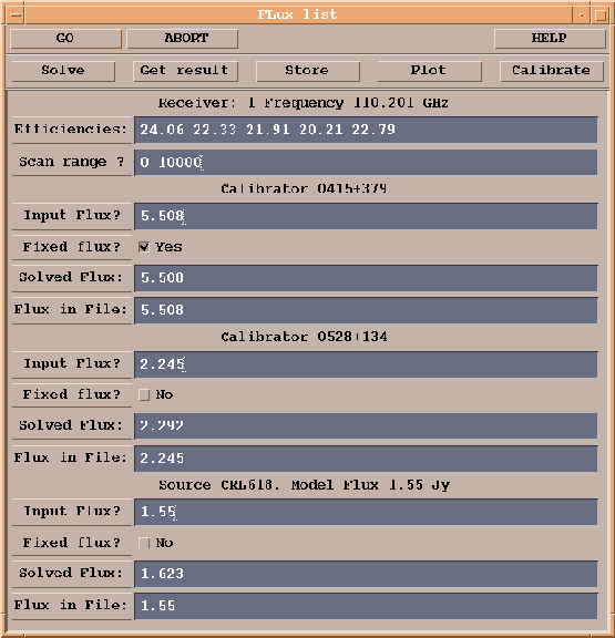
Fig.12.4 is a printout of the ``standard calibration procedure'' used in CLIC. This procedure uses the CLIC command SOLVE FLUX which works on cross-correlation only as follows:
In the automatic procedure, the reference sources are the calibrators where Fixed flux is set to YES and the reference values are in the variable Input Flux. Flux in file corresponds to the value stored with the data (by using the observational command FLUX, see Chapter 8 for details). The calculation is performed by clicking on SOLVE and the results are displayed inside the variable Solved Flux.
If you want to iterate using one of these values as reference, you
need to write it in the variable Input Flux and set Fixed flux to YES. Like in the CLIC command SOLVE
FLUX, the individual antenna efficiencies (
![]() ) are
computed; these values are only averaged values on the time
interval using all sources. They are then affected by many small
biases like pointing or focus errors and atmospheric decorrelation
and they are usually worse than the canonical values given in
table 12.2 (for biases, see end of this section).
) are
computed; these values are only averaged values on the time
interval using all sources. They are then affected by many small
biases like pointing or focus errors and atmospheric decorrelation
and they are usually worse than the canonical values given in
table 12.2 (for biases, see end of this section).
When you are satisfied by the flux calibration, you need to click
on the following sequence of buttons: 1) Get Results in
order to update the internal variables of the CLIC procedure, 2)
Store to save the flux values inside the header file
(hpb file) and 3) Plot to display the result of
your calibration. The plot shows the inverse of the antenna
efficiencies (
![]() ) versus time for all selected sources. If
the flux calibration is correct, all sources must have the same
value e.g.
) versus time for all selected sources. If
the flux calibration is correct, all sources must have the same
value e.g.
![]() . This plot is systematically done in
mode amplitude scaled (written on the top left corner). In
this mode, the antenna temperature of each source
. This plot is systematically done in
mode amplitude scaled (written on the top left corner). In
this mode, the antenna temperature of each source
![]() in K is divided by its assumed (variable Input flux) flux
density
in K is divided by its assumed (variable Input flux) flux
density ![]() in Jy (the value you have just stored), the
result is then
in Jy (the value you have just stored), the
result is then
![]() which
must be the same for all sources and equal to
which
must be the same for all sources and equal to
![]() . If it is
not the case, for example if one source appears systematically
lower or higher than the others, this means that its flux is wrong
and you need to iterate.
. If it is
not the case, for example if one source appears systematically
lower or higher than the others, this means that its flux is wrong
and you need to iterate.
Note that the scan range, applied on all calibrators, which is by default the scan range of the ``standard calibration procedure'' can be changed. This option is useful when there is some shadowing on one calibrator because the shadowing can strongly affect the result of a SOLVE FLUX. If you change the scan range, do not forget to click on UPDATE.
 |
In the final amplitude calibration performed on the source (see next section), the
flux of the source is determined by reference to the flux of the amplitude
calibrator which is usually also the phase calibrator. This means that the averaged
efficiencies
![]() computed by SOLVE FLUX and the automatic procedure are
not directly used and in many case variations of
computed by SOLVE FLUX and the automatic procedure are
not directly used and in many case variations of
![]() does not affect the
accuracy of the final amplitude calibration because they are corrected. It is then
fundamental to have a good estimate of the flux of the amplitude calibrator but not
necessarily to know precisely the averaged
does not affect the
accuracy of the final amplitude calibration because they are corrected. It is then
fundamental to have a good estimate of the flux of the amplitude calibrator but not
necessarily to know precisely the averaged
![]() .
.
Using the automatic procedure, the following biases may occur:
Note that the biases 3) and 4) do not affect flux estimates when they are performed on pointing data (as in sessions of flux measurements).
This program is not used by the external users of the PdBI but IRAM astronomers to provide reliable flux density of quasars to visitors (see flux reports). A description of the program is given in ``Flux measurement with the IRAM Plateau de Bure Interferometer'' by A.Dutrey & S.Guilloteau