Model fitting is the oldest way of analyzing interferometer data. It
was effectively used in the times where the coverage of the ![]() plane was too scarce to even think of creating an image by Fourier
transform. One assumes a simple source model depending of a few
parameters (source position, flux, size) and fits the visibility
function of that model to the visibility data. Of course one may use
a linear combination of several source models since the Fourier
transform is linear. This is performed using the GILDAS task UV_FIT. The result may be displayed with the procedure PLOTFIT. Both are available in the panel ``Interferometric UV
operations'' from the GRAPHIC standard menu.
plane was too scarce to even think of creating an image by Fourier
transform. One assumes a simple source model depending of a few
parameters (source position, flux, size) and fits the visibility
function of that model to the visibility data. Of course one may use
a linear combination of several source models since the Fourier
transform is linear. This is performed using the GILDAS task UV_FIT. The result may be displayed with the procedure PLOTFIT. Both are available in the panel ``Interferometric UV
operations'' from the GRAPHIC standard menu.
Table 14.1 gives examples of a few models and their visibility functions. For source models with a circular symmetry, the visibility function is split into a radial dependent amplitude and a phase factor which depends only on the source position.
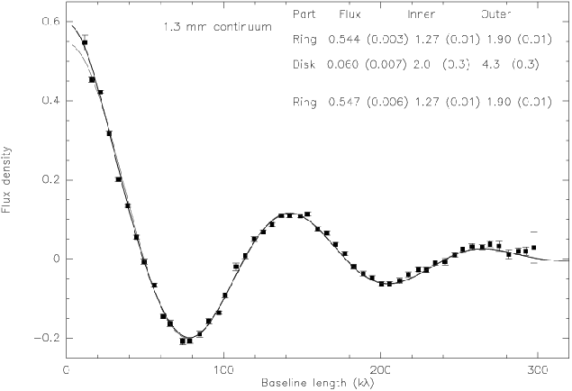
Some sources are actually so simple that this method may be used to a good accuracy (fig. 14.6).
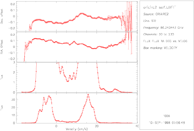
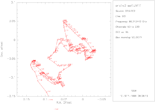
Quite often this method is used for sources that are unresolved or not well resolved at a given frequency; for instance a SiO maser may consist of several point-source components at different velocities. Fitting a point source in each channel one derives a ``spot map'' (figs 14.7,14.8).
For a source with central symmetry the task UV_CENTER determines the source position by using only the phases. Alternatively the task UV_FIT may be used to fit the amplitudes and phases at the same time, or e.g. to simultaneously fit a pair of sources.