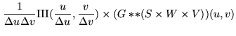
The combination of Gridding and Sampling produces the ![]() data set
data set
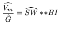
The Fourier Transform of this ![]() data set is
data set is
Accordingly, aliasing of ![]() in the map domain will thus occur.
Note at this stage that, providing aliasing of
in the map domain will thus occur.
Note at this stage that, providing aliasing of ![]() remains negligible, an exact convolution equation is preserved
remains negligible, an exact convolution equation is preserved
 |
(15.17) |
The gridding function will thus have to be selected to minimize
aliasing of ![]() . This criterion will depend on the image fidelity
required. Obviously, if the data is very noisy, aliasing of the
. This criterion will depend on the image fidelity
required. Obviously, if the data is very noisy, aliasing of the ![]() can be completely negligible.
can be completely negligible.
Furthermore, the weighting function ![]() is usually smooth, while the gridding
function
is usually smooth, while the gridding
function ![]() is a relatively sharp function (since it ensures the re-gridding by
convolution from nearby data points). Thus, to first order
is a relatively sharp function (since it ensures the re-gridding by
convolution from nearby data points). Thus, to first order
![]() ,
and we could rewrite Eq.15.14 as
,
and we could rewrite Eq.15.14 as
Let us focus on the choice of the gridding function. The gridding function will be selected according to the following principles:
The simplest gridding function is the Rectangular function
 |
(15.19) | ||
 |
(15.20) |
A better choice could be the Gaussian function
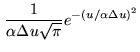 |
(15.21) | ||
| (15.22) |
However, a Gaussian still has fairly significant wings. ![]() should ideally be
a rectangular function (1 inside the map, 0 outside).
should ideally be
a rectangular function (1 inside the map, 0 outside). ![]() would be a sinc
function, but this falls off too slowly, and would require a lot of computations in
the gridding. Moreover, the (unavoidable) truncation of
would be a sinc
function, but this falls off too slowly, and would require a lot of computations in
the gridding. Moreover, the (unavoidable) truncation of ![]() would destroy the sharp
edges of
would destroy the sharp
edges of ![]() anyhow. Hence the idea to use an apodized version of the sinc function, the Gaussian-Sinc function
anyhow. Hence the idea to use an apodized version of the sinc function, the Gaussian-Sinc function
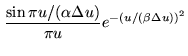 |
(15.23) | ||
| (15.24) |
The empirical approaches mentioned above do not guarantee any optimal choice of the
gridding function. A completely different approach is based on the desired
properties of the gridding function. We actually want ![]() to fall off as
quickly as possible, but
to fall off as
quickly as possible, but ![]() to be support limited. Mathematically, this defines a
class of functions known as Spheroidal functions. Spheroidal functions are
solutions of differential equations, and cannot be expressed analytically. In
practice, this is not a severe limitation since numerical representations can be
obtained by tabulating the gridding function values. Given the limited numerical
accuracy of the computations, the tabulation does not require a prohibitively fine
sampling of the gridding function, and is quite practical both in term of memory
usage and computation speed. Tabulated values are used in the task UV_MAP.
to be support limited. Mathematically, this defines a
class of functions known as Spheroidal functions. Spheroidal functions are
solutions of differential equations, and cannot be expressed analytically. In
practice, this is not a severe limitation since numerical representations can be
obtained by tabulating the gridding function values. Given the limited numerical
accuracy of the computations, the tabulation does not require a prohibitively fine
sampling of the gridding function, and is quite practical both in term of memory
usage and computation speed. Tabulated values are used in the task UV_MAP.
Note that the finite accuracy of the computation may ultimately limit the image dynamic range.