4.3.1 Digitization of the input signal and clipping correction

As already mentioned, sampling at the Nyquist rate retains all information. However, quantizing the input signal leads to a loss of information. This can be qualitatively understood in the following way: in order to reach the next discrete level of the transfer function, some offset has to be added to the signal. If the input signal is random noise of zero mean, the offset to be added will also be a random signal of zero mean. In other words, a ``quantization'' noise is added to the signal, that leads to a loss of information. In addition, the added noise is not anymore bandwidth limited, and the sampling theorem does not apply: oversampling will lead to improved sensitivity.

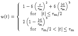
Many quantization schemes exist (see e.g. [Cooper 1970]). It is entirely sufficient to use merely a few quantum steps, if the cross-correlation function will be later corrected for the effects of quantization. For the sake of illustration, the transfer function of a four-level 2-bit quantization is shown in Fig.4.5. Each of the four steps is assigned a sign bit, and a magnitude bit. After discretizing the signal, the samples from one antenna are shifted in time, in order to compensate the geometric delay $\ensuremath{\tau_\mathrm{\scriptscriptstyle \rm G}} (t)$. The correlator now proceeds in the following way: for each delay step $\Delta t$, the corresponding sign and magnitude bits are put into two registers (one for the first antenna, and one for the second). The second register is successively shifted by one sample. In this way, sample pairs from both antennas, separated by a successively longer time lag, are created. These pairs are multiplied, using a multiplication table. For the case of four-level quantization, it is shown in Fig.4.5. Products which are assigned a value of $\pm{n}^2$ are called ``high-level products'', those with a value of $\pm{n}$are ``intermediate-level products'', and those with a value of $\pm{1}$``low-level products''. The products (evaluated using the multiplication table in Fig.4.5) are send to a counter (one counter for each channel, i.e. for each of the discrete time lags). After the end of the integration cycle, the counters are read out.

In practice, the multiplication table will be shifted by a positive offset of n², to avoid negative products (the offset needs to be corrected when the counters are read out). This is because the counter is simply an adding device. As another simplification, low-level products may be deleted. This makes digital implementation easier, and accounts for a loss of sensitivity of merely 1% (see Table 4.1). Finally, not all bits of the counters' content need to be transmitted (see Section3.3.2).

Before the normalized contents of the counters are Fourier-transformed, they need to be corrected, because the cross-correlation function of quantized data does not equal the cross-correlation function of continuous data. This ``clipping correction'' can be derived using two different methods. As an example for the case of full 4-level quantization:

• Four-level cross-correlation coefficient according to the multiplication table Fig.4.5. The cross-correlation coefficient $\rho$ is a normalized form of the cross-correlation function (see AppendixA):
  

  $$\rho_4 = \frac{2n^2(N_{01,01}-2N_{01,11})+4n(N_{00,01}-N_{00,... ...+2(N_{00,00}-N_{00,10})}{2(n^2N_{01,01}+N_{00,00})_{\rho = 1}}$$ (4.8)

  
  
  where $N_{\rm ij,kl}$ is the number of counts with sign bit i and magnitude bit j at time t (first antenna), and sign bit k and magnitude bit l at time $t+\tau$ (second antenna). $\pm{n}$ is the product value assigned to intermediate-level products.
• Clipping correction, first method: evaluate the $N_{\rm ij,kl}$ in Eq.4.9, using joint probabilities $P_{\rm ij,kl}$ (see AppendixA for the definition of the jointly Gaussian probability distribution), such as
  

  $$N_{01,01} = NP_{01,01} = \frac{N}{2\pi\sigma^2\sqrt{1-\rho^2}... ...[\frac{-(x^2+y^2-2\rho xy)}{2\sigma^2(1-\rho^2)}\right]}dx}dy}$$ (4.9)

  
  
  (N is the number of signal pairs, separated by the time lag of the channel under consideration, v₀ is the clipping voltage, see Fig.4.4).
• Clipping correction, second method: using Price's theorem for functions of jointly random variables. The result, derived in AppendixB, is shown in Fig.4.4:
  
   

  $$\frac{\sigma^2}{\pi}\int_{0}^{\rho}{ \frac{1}{\sqrt{1-r^2}}\biggl\{(... ...\sigma^2(1+r)}\right)}+ \exp{\left(\frac{-v_0^2}{\sigma^2(1-r)}\right)}\right]}$$ R₄ =

  $${+4(n-1)\exp{\left(\frac{-v_0^2}{2\sigma^2(1-r^2)}\right)}+2\biggr\}dr}\,.$$ (4.10)

  
  

Although the discrete, normalized cross-correlation function and the continuous cross-correlation coefficient are almost linearly dependent within a wide range, the correction is not trivial. An analytical solution is only possible for the case of two-level quantization (``van Vleck correction''  [Van Vleck 1966]).

In practice, several methods are used to numerically implement Eq.4.11 (in the following, the index k means k-level quantization). The integrand may be replaced by an interpolating polynomial, allowing to solve the integral. One may also construct an interpolating surface $\rho(R_{\rm k},\sigma)$. As already discussed, the clipping correction cannot recover the loss of sensitivity due to quantization. The loss of sensitivity for k-level discretization may be found by evaluating the signal-to-noise ratio

$$\Re_{{\rm sn},k}= \frac{R_{\rm k}}{\sigma_k} = \frac{R_{\rm k}}{\sqrt{\langle R_k^2\rangle - \langle R_k \rangle^2}}$$ (4.11)

In order to minimize the loss of sensitivity, the clipping voltage (with respect to the noise $\sigma$) needs to be adjusted such that the correlator efficiency curve in Fig.4.4 is at its maximum. The correlator efficiency is defined with respect to the signal-to-noise ratio of a (fictive) continuous correlator, i.e.

$$\eta_k = \frac{\Re_{{\rm sn},k}}{\Re_{\rm sn,\infty}} = \frac{\Re_{{\rm sn},k}}{\rho\sqrt{N_{\rm q}}}$$ (4.12)

where $N_{\rm q}$ is the number of samples. Table4.1 summarizes the results for different correlator types and samplings.

Due to the discretization of the input voltages (as shown in Fig.4.5), any knowledge of the absolute signal value is lost. The signal amplitude is recovered by a regularly performed calibration (using a calibration load of known temperature, for details, see the lecture by A.Dutrey).

  

Figure 4.4: Left: Clipping correction (cross correlation coefficient of a continuous signal vs. cross correlation correlation coefficient of a quantized signal) for two-, three- and four level quantization (with optimized threshold voltage). The case of two level quantization is also known as van Vleck correction. For more quantization levels, the clipping correction becomes smaller. Right: Correlator efficiency as function of the clipping voltage, for three-level and four-level quantization (at Nyquist sampling).

  

Figure: Left: Transfer function for a 4-level 2-bit correlator. The dashed line corresponds to the transfer function of a (fictive) continuous correlator with an infinite number of infinitesimally small delay steps. Right: Multiplication table. S(x) is the signal bit at time t, M(x) is the magnitude bit at time t (respectively S(y) and M(y) at time $t+\tau$).

 

Table 4.1: Correlator parameters for several quantization schemes

method	n	v0 [ $\sigma_{\rm rms}$]	$\eta_{\rm q}^{(1)}$ for
			sampling rate
			$2\Delta\ensuremath{\nu_\mathrm{\scriptscriptstyle IF}} ^{(2)}$	$4\Delta\ensuremath{\nu_\mathrm{\scriptscriptstyle IF}} ^{(3)}$
two-level	-	-	0.64	0.74
three-level	-	0.61	0.81	0.89
four-level	3	1.00	0.88(4)	0.94
	4	0.95	0.88	0.94
$\infty$-level	-	-	1.00	1.00

Notes:
(1) The correlator efficiency is defined by Eq.4.13.
The values are for an idealized (rectangular)
bandpass and after level optimization.
(2) Nyquist sampling,
(3) oversampling by factor 2
(4) 0.87 if low level products deleted
(case of Plateau de Bure correlator)  

 

Table 4.2: Time lag windows

Description	Lag window	Spectral window
rectangular	w(t) = 1 for $\vert t\vert \le \tau_{\rm m}$, else 0	$\hat{w}(\nu) = 2\tau_{\rm m}\frac{\sin{(2\pi\nu \tau_{\rm m})}}{2\pi\nu\tau_{\rm m}}$
Bartlett	$w(t) = 1-\frac{\vert t\vert}{\tau_{\rm m}}$ for $\vert t\vert \le \tau_{\rm m}$, else 0	$\hat{w}(\nu) = \tau_{\rm m} \left(\frac{\sin{(\pi\nu\tau_{\rm m})}}{\pi\nu\tau_{\rm m}}\right)^2$
von Hann	$w(t) = \frac{1}{2}\left(1+\cos{(\frac{\pi t}{\tau_{\rm m}})} \right)$ for $\vert t\vert \le \tau_{\rm m}$, else 0	$\hat{w}(\nu) = \tau_{\rm m}\cdot\frac{\sin{(2\pi\nu\tau_{\rm m})}} {2\pi\nu\tau_{\rm m}}\cdot\frac{1}{1-(2\nu\tau_{\rm m})^2}$
Welch	$w(t) = \left(1-(\frac{t}{\tau_{\rm m}})^2\right)$	$\hat{w}(\nu) = \frac{1}{(\pi\nu)^2\tau_{\rm m}}\left( \frac{\sin{(2\pi\nu\tau_{... ...nu\tau_{\rm m}}-{\mbox{\small cos}\mbox{\small$(2\pi\nu\tau_{\rm m})$ }}\right)$
Parzen	$w(t) = \left\{ \begin{array}{l} 1-6\left(\frac{t}{\tau_{\rm m}}\right)^2+6\lef... ...rm{for}~~~ \tau_{\rm m}/2 < \vert t\vert \le \tau_{\rm m} \end{array} \right.$	$\hat{w}(\nu) = \frac{3}{4}\tau_{\rm m} \left(\frac{\sin{(\pi\nu\tau_{\rm m}/2)}}{\pi\nu\tau_{\rm m}/2}\right)^4$