4.3.2 Time lag windows and spectral resolution

According to the sampling theorem, we can recover the cross-power spectral density within a bandwidth $\Delta\ensuremath{\nu_\mathrm{\scriptscriptstyle IF}} = 1/(2\Delta t)$, if the sampling step is $\Delta t$. The channel spacing $\delta\nu$ is then determined by the maximum time lag $\tau_{\rm max} = N_{\rm ch}\Delta t$(where $N_{\rm ch}$ is the number of channels), i.e.

$$\delta\nu = \frac{1}{2\tau_{\rm max}} = \frac{1}{2N_{\rm ch}\Delta t}$$ (4.13)

However, the data acquisition is abruptly stopped after the maximum time lag. After the Fourier transform, the observed cross power spectrum is convolved with the Fourier transform $\hat{w}(\nu)$ of the box-shaped time window w(t), producing strong sidelobes:

$$w(\tau) = \left\{ \begin{array}{ll} 1, & \vert\tau\vert \le \tau_... ...au_{\rm max})}}{2\ensuremath{\nu_\mathrm{\scriptscriptstyle }}\tau_{\rm max}}\;$$ (4.14)

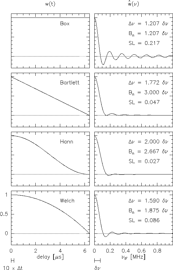
These oscillations are especially annoying, if strong lines are observed. They may be minimized, if the box-shaped time lag window is replaced by a function that rises from zero to peak at negative time lags, and decreases to zero at positive time lags (apodization). Such a window function suppresses the sidelobes, at the cost of spectral resolution. A comparison between several window functions is given in Fig.4.6, together with sidelobe levels and spectral resolutions (defined by the FWHP of the main lobe of the spectral window). Table 4.2 summarizes the various functions in time and spectral domains. The default of the Plateau de Bure correlator is the Welch window, because it still offers a good spectral resolution. Moreover, the oscillating sidelobes partly cancel out the contamination of a channel by the signals in adjacent channels. Of course, the observer is free to deconvolve the spectra from this default window, and to use another time lag window.
Note: If you apodize your data, not only the effective spectral resolution is changed. Due to the suppression of noise at large time lags, the sensitivity is increased. The variance ratio of apodized data to unapodized data,

$$\int_{-\infty}^\infty{\vert w(t)\vert^2dt} = \int_{-\infty}^\infty{\vert\hat{w}(\nu)\vert^2d\nu} = 1/B_{\rm n}$$ (4.15)

defines the noise equivalent bandwidth $B_{\rm n}$. It is the width of an ideal rectangular spectral window (i.e. $\hat{w}(\nu) = 1/B_{\rm n}$ with zero loss inside $\vert\nu\vert \le B_{\rm n}/2$, and infinite loss outside) containing the same noise power as the actual data. For sensitivity estimates of spectral line observations, the channel width to be used is thus the noise equivalent width, and neither the channel spacing, nor the effective spectral resolution. For commonly used time windows, Fig.4.6 gives the noise equivalent bandwidths.

  

Figure: Several time lag windows, and their Fourier transforms (normalized to peak). The sidelobe levels SL are indicated, as well as the spectral resolution (defined as the FWHP of the main lobe), and the noise equivalent width. The delay stepsize, and channel spacing are indicated for the following example: 256 channels, clock rate 40MHz, resulting in a channel spacing of 78.125kHz.