10.5 Phase fluctuation evaluation

10.5.1 Cause of Phase Fluctuations

The phase measured by an interferometer is the difference in the arrival times of the signals at the different antennas. The phase difference contains useful information about the location and structure of the source, but is also affected by atmospheric inhomogeneities. The complex dielectric constant fluctuates in time and in space as the distributions of water droplets, ice particles, and atmospheric gases suffer variations. In the case of clear atmosphere (no scatterers present) the main source of phase delay is water vapor. When there is more water vapor along the optical path of one of the telescopes, the incoming radiation will experience an additional delay and the measured phase will increase by $\Delta \phi$. With wind the amount of water vapor in the beam of each telescope will change over time and so will the detected phase. This phase delay has a resonant behavior as seen in section 10.2.4. As a result, the source appears to move around in the sky and, if the signals are integrated over a period of time which is long compared to the time scale of the fluctuations (few to tens of seconds), resolution as well as signal strength will be degraded. Fluctuations in the dry component of the atmosphere can also originate phase delays but these are in general less important.

10.5.2 Simulations of phase fluctuations

Figure 10.5: Upper panel: Derivative of the phase delay respect to the water vapor column (differential phase in text; this derivative is independent of the water vapor column) as a function of frequency, superposed on the Chajnantor atmospheric transmission curve for 0.3 mm of water vapor. Lower panel: Derivative of the phase delay respect to the sky brightness temperature for 0.3 mm H$_{2}$O column.

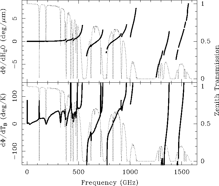
Present day radio interferometers are mostly limited to frequencies below 350 GHz. Phase delay increases in importance as the frequency increases into the submillimeter domain because of the strength of the atmospheric lines involved in both absorption and dispersion. Using the complex line shape of equation 10.22 we have calculated the derivative of the phase delay respect to the water vapor column $\frac{\partial\phi}{\partial N_{H_{2}O}}$ (this derivative will be called the differential phase and is provided in deg/$\mu$m here). The differential phase as a function of frequency has been plotted for the Chajnantor site in Figure 10.5 (where the curve is restricted to those frequencies where the transmission is above 10% when the precipitable water vapor column is 0.3 mm, i.e. very good conditions for single-dish submillimeter observations). Another useful quantity plotted in the same figure is the derivate of the phase delay with respect to the sky brightness temperature (T$_{B,sky}$), since this function relates the phase correction between two antennas to a measurable physical parameter (T$_{B,sky}$). Note however that whereas the differential phase described above depends only on $\Delta N_{H_{2}O}$, this new quantity depends on $N_{H_{2}O}$ as well. The curve plotted here corresponds to $\frac{\partial\phi}{\partial T_{b}}(\nu)$ at $N_{H_{2}O}$=0.3mm.

As seen in Figure 10.5, the differential phase becomes much more important in the submillimeter domain than it is at millimeter wavelengths, so its correct estimation and the selection of the best means of monitoring water vapor column differences between different antennas are essential for the success of ground-based submillimeter interferometry. For example, the differential phase is 0.0339 deg/$\mu$m at 230 GHz whereas it is -0.4665 and 0.2597 deg/$\mu$m at 650 and 850 GHz respectively, roughly an order of magnitude larger.

Figure 10.6: Phase correction results for the CSO-JCMT interferometer using 183.31 GHz 3-channel water vapor monitors (courtesy of Martina Wiedner).

10.5.3 Phase Correction Methods

There are basically two different phase correction methods:

A) The phase offset due to the atmosphere can be measured directly by observing a calibrator, i.e., a strong point source whose position and hence theoretical phase are well known. Assuming instrumental errors are small the difference between the measured and the theoretical phase gives the phase offset introduced by the atmosphere. The phase offsets, which are interpolated between measurements on the calibrator, are subtracted from the measured phase of an astronomical source.

B) The correction can be determined indirectly by detecting the emission from water molecules and calculating the phase error from the differences in the amounts of water along the paths to the individual antennas using a model as presented on Figure 10.5. There are two different approaches to determine the amount of water vapor: (i) Total Power Method, where the astronomical receivers measure the continuum emission; and (ii) Radiometric Phase Correction, where the emission from water lines is measured by dedicated instruments. So far, radiometers monitoring the 22 GHz and the 183 GHz lines have been built and tested. Receivers at 22 GHz typically have lower noise temperatures than those at 183 GHz, but on (very) dry sites, such as Chajnantor, the 183 GHz monitors will be ideal to measure the optical path with higher accuracy due to the much higher conversion factors from sky brightness temperature in K to optical path length in mm.

10.5.4 Example of phase correction

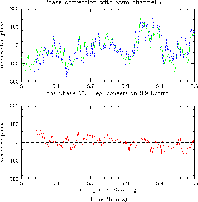
Fig. 10.6 shows typical phase correction results in normal night time weather for Mauna Kea (2.2 mm $N_{H_{2}O}$): The CSO-JCMT interferometer observed bright hydrogen recombination line maser emission towards the source MWC349 at 354 GHz. The solid curve in the top plot displays the measured phase after Doppler correction, it represents the atmospheric phase fluctuations and some electronic phase noise. The dashed line shows the phase predicted by the water vapor monitors. The measured and the predicted phase agree well and their difference is plotted in the lower graph. Phase correction reduces the rms phase fluctuations from $60^\circ$ (140 $\mu$m) to $26^\circ$ (60 $\mu$m) over 30 minutes. If one would integrate on source for 30 minutes 42% of the astronomical flux would be lost due to decorrelation, but with phase correction the loss would amount to only 10%.