12.2 Single-dish Calibration of the Amplitude

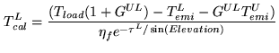
The goal of this part of the calibration is to measure the atmospheric transparency above each antenna.

This calibration is done automatically and in real-time but it can be redone a posteriori if one or several parameters are wrong using the CLIC command ATMOSPHERE. However, for 99 % of the projects, the single-dish calibration is correct. Moreover, we will see in this section that in most cases, even with erroneous calibration parameters, it is almost impossible to do an error larger than $\sim 5\%$.

For details about the properties of the atmosphere, the reader has to refer to Chapter 11 while the transmission of the atmosphere at mm wavelengths is described in Chapter 10. Most of this lecture is extracted from the documentation ``Amplitude Calibration'' by [Guilloteau 1990] for single-dish telescope and from [Guilloteau et al. 1993].

Since all this part of the calibration is purely antenna dependent and in order to simplify the equations, the subscript $_i$ will be systematically ignored. In the same spirit, the equations will be expressed in $T_A^*$ scale taking $\eta_f=\eta_b$ (see [Guilloteau 1990]).

The atmospheric absorption (e.g. for the lower side-band $T_{cal}^L$) can be expressed by

$$T_{cal}^L = \frac{(T_{load}(1+G^{UL})-T_{emi}^L-G^{UL}T_{emi}^U)} {\eta_f e^{-\tau^L/\sin(Elevation)}}$$ (12.5)

where $T_{load}$ is the hot load and $T_{emi}^L$ and $T_{emi}^U$ are the noise temperature received from the sky in the lower an upper sidebands respectively (for the IRAM interferometer, the difference in frequency between the upper and lower sidebands is $\sim3$ GHz).

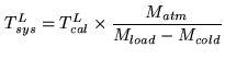
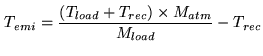
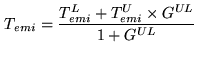
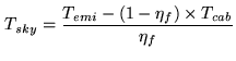
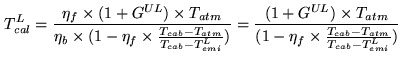
The system temperature $T_{sys}$ is given by:

$$T_{sys}^L = T_{cal}^L\times \frac{M_{atm}}{M_{load}-M_{cold}}$$ (12.6)

The main goal of the single-dish calibration is to measure $T_{cal}$ (hence $T_{sys}$) as accurately as possible.

At Bure, during a standard atmospheric calibration, the measured quantities are:

• Phase 1, $M_{atm}$: the power received from the sky
• Phase 2, $M_{load}$: the power received from the hot load
• (Phase 3), $M_{cold}$: the power received from the cold load

$T_{rec}$, the noise temperature of the receiver, is deduced from the measurements on the hot and cold loads at the beginning of each project and regularly checked. The phase 2 (hot load) is also not systematically done (this remains valid because temperature drifts on the hot load are on timescales of several hours). The receiver sideband ratio $G^{UL}$ is also measured at the beginning of each project (see Chapter 9). $T_{emi}$, the effective temperature seen by the antenna, is given by

$$T_{emi} =\frac{(T_{load}+T_{rec}) \times M_{atm}}{M_{load}}-T_{rec}$$ (12.7)

Moreover, $T_{emi}$ which is measured on the bandwidth of the receiver, can be expressed as the sum of $T_{emi}^L$ and $T_{emi}^U$ (a similar expression exists for $T_{sky}$):

$$T_{emi}= \frac{T_{emi}^L+T_{emi}^U \times G^{UL}}{1+G^{UL}}$$ (12.8)

$T_{emi}$ is directly linked to the sky temperature emissivity (or brightness temperature) $T_{sky}$ by:

$$T_{sky} = \frac{T_{emi}- (1-\eta_f)\times T_{cab}}{\eta_f}$$ (12.9)

were $T_{cab}$ is the physical temperature inside the cabin and $\eta_f$, the forward efficiency, which are both known (or measurable) quantities.

Our calibration system provides then a direct measurement of $T_{emi}$ and hence of $T_{sky}$, which is deduced from quantities accurately measured. Hence, in Eq.12.5 the only unknown parameter remains $\tau^L$, the opacity of the atmosphere at zenith, which is iteratively computed together with $T_{atm}$ the physical atmospheric temperature of the absorbing layers. This calculation is performed by the atmospheric transmission model ATM (see Chapter 10) and the documentation ``Amplitude Calibration'').

The opacity $\tau^L$ (or more generally $\tau_\nu$) comes from two terms:

$$\tau_\nu = A_\nu + B_\nu \times w$$ (12.10)

$A_\nu$ and $B_\nu$ are the respective contributions to O$_2$ and H$_2$O, the water vapor content $w$ is then adjusted with $T_{atm}$ by the model ATM to match the measured $T_{sky}$. The ATM model works as long as the hypothesis done on the structure of the atmosphere in plane-parallel layers is justified, as it is usually the case for standard weather conditions.

12.2.1 Low opacity approximation and implication for $T_{cal}$

When the opacity of the atmosphere is weak ( $\tau_\nu < 0.2$) and equal in both image and signal bands, $T_{cal}$ is mostly dependent of $T_{atm}$ and both of them can be considered as independent of $\tau_\nu$ and hence $w$.

In the conditions mentioned above, $\tau_\nu$ can be eliminated from Eq.12.5. The equation becomes:

$$T_{cal}^L = \frac{\eta_f \times (1+G^{UL})\times T_{atm}} {\eta_b... ...UL})\times T_{atm}} {(1-\eta_f\times\frac{T_{cab}-T_{atm}}{T_{cab}-T_{emi}^L})}$$ (12.11)

(details about the derivation of Eq.12.11 are given in the documentation ``Amplitude Calibration'' by S.Guilloteau). In Eq.12.11, the unknown is $T_{atm}$, the physical temperature of the absorbing layers. $T_{atm}$ is mostly dependent on the outside temperature, pressure and site altitude and weakly on $\tau_\nu$. For this reason, $T_{cal}$ and $T_{sys}$ remain correct even if $w$ and hence $\tau_\nu$ are not properly constrained.

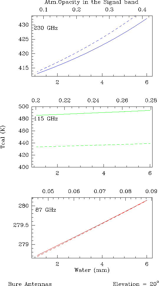
Figures 12.1 and 12.2 illustrate this point. Thick lines correspond to the exact equation (Eq.12.5) and dashed lines to the approximation (Eq.12.11). The comparison between Eq.12.11 and 12.5 was done for three common cases 1) at 87 GHz, with $G^{UL}=10^{-2}$, 2) at 115 GHz, with $G^{LU}=0.5$ and at 230 GHz, with $G^{UL}=0.5$. For the 15-m dishes, the forward efficiencies used are $\eta_f =0.93$ at 3mm and $\eta_f = 0.89$ at 1.3mm. Fig.12.1 is done for a source at $elevation=20^0$ and Fig.12.2 for a source at $elevation=60^o$.

Figure 12.1: Calibration temperature as function of water vapor (or opacity) at 87, 115 and 230 GHz for a source at 20 degrees elevation. Parameters are taken for the Bure interferometer (see text). Thick lines correspond to the exact equation (Eq.12.5) and dashed lines to the approximation (Eq.12.11).

Figure 12.2: Calibration temperature as function of water vapor (or opacity) at 87, 115 and 230 GHz for a source at 60 degrees elevation. Parameters are taken for the Bure interferometer (see text). Thick lines correspond to the exact equation (Eq.12.5) and dashed lines to the approximation (Eq.12.11).

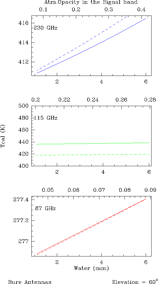The following points can be deduced from these figures:

1. As long as $T_{sky}^L=T_{sky}^U$, the equation 12.11 remains valid even at high frequencies $> 200$ GHz and for $w> 5$ mm.
2. This comes from the fact the $T_{atm}$ is mostly independent of the atmospheric water vapor content.
3. As soon as $T_{sky}^L \neq T_{sky}^U$, the equation 12.11 is not valid. Note also that the error is about constant with the opacity because $T_{atm}$ is mostly independent of the atmospheric water vapor content. Moreover at 115 GHz, the atmospheric opacity is dominated by the 118 GHz Oxygen line and cannot be below 0.2 and the amount of opacity added by the water vapor is small. $T_{cal}$ remains mostly constant with $w$.

At mm wavelengths, the derivation of the $T_{cal}$ (or $T_{sys}$) using an atmospheric model is then quite safe.

12.2.2 Absolute errors on $T_{cal}$ due to instrumental parameters

The equations above show that $T_{cal}$ is also dependent of the instrumental parameters $T_{rec}$, $\eta_f$ and $T_{load}$. These parameters can also lead to errors on $T_{cal}$. Derivatives of the appropriate equations are given in the IRAM report ``Amplitude Calibration''. Applying these equations and taking $T_{atm}=240$ K, $T_{load}=290$ K and $T_{emi}=50$ K, the possible resulting errors are given in the table 12.1.

Table 12.1: Percentage error on amplitude scale introduced by erroneous input parameters.

Item	$T_{cab}$	$T_{rec}$	$\eta_{f}$
Typical Error	2 K	10 K	0.01
Induced variation (in %)	0.7	0.3	1.3

As a consequence, the most critical parameter of the calibration is the Forward Efficiency $\eta_f$. This parameter is a function of frequency, because of optics surface accuracy, but also of the receiver illumination. If $\eta_f$ is underestimated, $T_{sky}$ is underestimated and you may obtain anomalously low water vapor content, and vice-versa.

The sideband gain ratio $G^{UL}$ is also a critical parameter. $G^{UL}$ is not only a scaling factor (see Eq.12.5), but is also involved in the derivation of the atmospheric model since the contributions from the atmosphere in image and signal bands are considered. This effect is important only if the opacities in both bands are significantly different, as for the J=1-0 line of CO.

Eq.12.5 shows that as soon as the receivers are tuned in single side band ( $G^{UL}<10^{-2}$ or rejection $>20$dB), the effect on $T_{cal}^L$ is insignificant. Errors can be significant when the tuning is double-side band with values of $G^{UL}$ around $\sim 0.8-0.2$. For example, when the emissivity of the sky is the same in both bands ( $T_{sky}^U=T_{sky}^L$), the derivative of Eq.12.8 shows that an error of 0.1 on $G^{UL}=0.5$ leads to $\frac{\Delta T_{cal}}{T_{cal}}\simeq \frac{dG^{UL}}{1+G^{UL}} \sim 6.5\%$.

However, this problem is only relevant to single-dish observations and should not happen in interferometry because as soon as three antennas are working, $G^{UL}$ can be accurately measured (see Chapter 9). At Bure the accuracy on $G^{UL}$ is better than about 1 % and the system is stable on scale of several hours.

12.2.3 Relative errors or errors on $T_{cal}^L/T_{cal}^U$

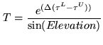
Following Eq.12.5, the side band ratio will be affected by the following term:

$$T = \frac{e^{(\Delta(\tau^L-\tau^U))}}{\sin (Elevation)}$$ (12.12)

where $\Delta(\tau^L-\tau^U)$ is the error on the sideband zenith opacity difference. This difference is maximum at frequencies corresponding to a wing of an atmospheric line, for example when observing around 115 GHz, near the O$_2$ line at 118 GHz. As example, taking the frequencies of 112 and 115 GHz for a source at $20^o$ in elevation and a zenith opacity difference $(\tau^L-\tau^U)=0.150$, an error of 0.030 on this difference (coming from $A_\nu$) will give an error of less than 1% on the gain $G^{UL}$. Moreover errors on Oxygen lines are very unlikely because the content in Oxygen in the atmosphere is relatively well known and only varying with the altitude of the site.

At the same frequencies, an error of 5mm (which would be enormous) on the water vapor content will only induce an error of 1% on the gain. Around such low frequency and for small frequency offsets, the water absorption is essentially achromatic. Improper calibration of the water vapor fluctuations will then result in even smaller errors since this is a random effect.

12.2.4 Estimate of the thermal noise

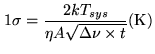
The resulting thermal noise is given by

$$1 \sigma = \frac{2 k T_{sys}}{\eta A \sqrt{\Delta \nu \times t}} (\mathrm{K})$$ (12.13)

where $k$ is the Boltzmann's constant, A is the geometric collecting area of the telescope, $\eta$ the global efficiency factor (including decorrelation, quantization, etc...), $\Delta \nu$ the bandwidth in use and $t$ the integration time. The resulting error on the phase determination is inversely proportional to the signal to noise ratio, as shown in Fig.12.3.

Figure 12.3: Phase error resulting from limited S/N ratio. $\sigma _\phi \approx 1/(S/N)$.