In the previous section we have considered a monochromatic system. We have actually finite bandwidths and in principle the gain coefficients are functions of both frequency and time. We thus write:
| (9.11) |
| (9.12) |
| (9.13) |
Frequency dependence of the gains occurs at several stages in the
acquisition chain. In the correlator itself the anti-aliasing
filters have to be very steep at the edges of each subband. A
consequence is that the phase slopes can be high there too. Any
non-compensated delay offset in the IF can also be seen as a phase
linearly dependent on frequency. The attenuation in the cables
strongly depends on IF frequency, although this is normally
compensated for, to first order, in a well-designed system. The
receiver itself has a frequency dependent response both in amplitude
and phase, due the IF amplifiers, the frequency dependence on the
mixer conversion loss. Antenna chromatism may also be important.
Finally the atmosphere itself may have some chromatic behavior, if
we operate in the vicinity of a strong line (e.g. O![]() at 118 GHz)
or if a weaker line (e.g. O
at 118 GHz)
or if a weaker line (e.g. O![]() ) happens to lie in the band.
) happens to lie in the band.
Bandpass calibration usually relies on observing a very strong source for some time; the bandpass functions are obtained by normalizing the observed visibility spectra by their integral over frequency. It is a priori not necessary to observe a point source, as long as its visibility can be assumed to be, on all baselines, independent on frequency in the useful bandwidth. If there is some dependence on frequency, then one should take this into account.
In many cases the correlator can be split in several independent subbands that are centered to different intermediate frequencies, and thus observe different frequencies in the sky. In principle they can be treated as different receivers since they have different anti-aliasing filters and different delay offsets, due to different lengths of the connecting cables. Thus they need independent bandpass calibrations, which can be done simultaneously on the same strong source.
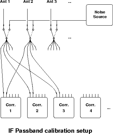
At millimeter wavelengths strong sources are scarce, and it is more practical to get a relative calibration of the subbands by switching the whole IF inputs to a noise source common to all antennas (Fig. 9.1). The switches are inserted before the IFs are split between subbands so that the delay offsets of the subbands are also calibrated out. This has several advantages: the signal to noise ratio observed by observing the noise source is higher than for an astronomical source since it provides fully correlated signals to the correlator; then such a calibration can be done quite often to suppress any gain drift due to thermal variations in the analogue part of the correlator. Since the sensitivity is high, this calibration is done by baseline, so that any closure errors are taken out.
When such an ``IF passband calibration'' has been applied in real time, only frequency dependent effects occurring in the signal path before the point where the noise source signal is inserted remain to be calibrated. Since at this point the signal is not yet split between subbands, the same passband functions are applicable to all correlator subbands.
At Plateau de Bure an ``IF passband calibration'' is implemented. Of course when the noise source is observed the delay and phase tracking in the last local oscillators (the one in the correlator IF part) are not applied.
The precision in phase is
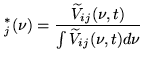
To actually determine the functions
![]() we observe a strong source,
with a frequency-independent visibility.
The visibilities are
we observe a strong source,
with a frequency-independent visibility.
The visibilities are
| (9.14) |
 |
(9.15) |
The passband calibrated visibility data will then be:
| (9.16) |
The most important here is the phase precision: it sets the uncertainty for relative positions of spectral features in the map. A rule of thumb is:
| (9.17) |
The amplitude accuracy can be very important too, for instance when
one wants to measure a weak line in front of a strong continuum, in
particular for a broad line. In that case one needs to measure the
passband with an amplitude accuracy better than that is needed on
source to get desired signal to noise ratio. Example: we want to
measure a line which is ![]() of the continuum, with a SNR of 20 on
the line strength; then the SNR on the continuum source should be
200, and the SNR on the passband calibration should be at least as
good.
of the continuum, with a SNR of 20 on
the line strength; then the SNR on the continuum source should be
200, and the SNR on the passband calibration should be at least as
good.
A millimeter-wave interferometer can be used to record separately the signal in both sidebands of the first LO (see Chapter 7). If the first mixer does not attenuate the image sideband, then it is useful to average both sidebands for increased continuum sensitivity, both for detecting weaker astronomical sources and increasing the SNR for calibration.
However the relative phases of the two sidebands can be arbitrary (particularly at Plateau de Bure where the IF frequency is variable since the LO2 changes in frequency in parallel with the LO1). This relative phase must be calibrated out. This it is done by measuring the phases of the upper and lower sidebands on the passband calibrator observation. These values can be used later to correct each sideband phase to compensate for their phase difference.
During the passband calibration one calculates:
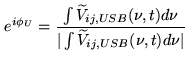 |
(9.18) |
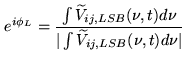 |
(9.19) |
| (9.20) |
At observing time, offsets on the first and second LOs can be
introduced so that both ![]() and
and ![]() are very close to zero
when a project is done. This actually done at Plateau de Bure, at
the same time when the sideband gain ratio is measured (see Chapter 12).
are very close to zero
when a project is done. This actually done at Plateau de Bure, at
the same time when the sideband gain ratio is measured (see Chapter 12).